Want to become an expert in VBA? So this is the right place for you. This blog mainly focus on teaching how to apply Visual Basic for Microsoft Excel. So improve the functionality of your excel workbooks with the aid of this blog. Also ask any questions you have regarding MS Excel and applying VBA. We are happy to assist you.

Open an outlook email and populate the body of the email


             Today I'm going to explain you how to generate Outlook email and populate with the required details of a worksheet automatically using VBA.                                                          
Here below is a example worksheet. It contains ID1, Email Addess, First name and Data.
And there is a button call "E-mail" in that sheet. What we need to do is Once we click the button it should  ask us to enter row number of data we want to email. When we input that number and press OK, Message should be opened with required data.


So first we need to get the row number from the user.


Dim RowNo As Integer
RowNo = InputBox("Please enter the row number you need to email:", "")


So it will show this input box.


Then we need to create the body of the email.

Dim WS As Worksheet
Dim messageBody As String

Set WS = ActiveSheet

messageBody = "Dear " & WS.Range("C" & RowNo) & "," & vbCrLf & vbCrLf & _
"Your ID1: " & WS.Range("A" & RowNo) & vbCrLf & vbCrLf & _
"Your email address: " & WS.Range("B" & RowNo) & vbCrLf & vbCrLf & _
"Your data: " & WS.Range("D" & RowNo) & vbCrLf & vbCrLf & _
"Please store this information in a safe place." & vbCrLf & vbCrLf & _
"Kind regards," & vbCrLf & vbCrLf & _
"Paul"

So message will be constructed similar to below.

Finally we need to create the outlook mail. Below code will do that part.

Dim OutApp As Outlook.Application
Dim objMsg As MailItem

Set OutApp = CreateObject("Outlook.Application")
Set objMsg = OutApp.CreateItem(olMailItem)

With objMsg
  .Body = messageBody
  .Display
End With

And here is the full code for this automation.


Dim RowNo As Integer
RowNo = InputBox("Please enter the row number you need to email:", "")
Dim WS As Worksheet
Dim messageBody As String
Set WS = ActiveSheet
messageBody = "Dear " & WS.Range("C" & RowNo) & "," & vbCrLf & vbCrLf & _
"Your ID1: " & WS.Range("A" & RowNo) & vbCrLf & vbCrLf & _
"Your email address: " & WS.Range("B" & RowNo) & vbCrLf & vbCrLf & _
"Your data: " & WS.Range("D" & RowNo) & vbCrLf & vbCrLf & _
"Please store this information in a safe place." & vbCrLf & vbCrLf & _
"Kind regards," & vbCrLf & vbCrLf & _
"Paul"
Dim OutApp As Outlook.Application
Dim objMsg As MailItem
Set OutApp = CreateObject("Outlook.Application")
Set objMsg = OutApp.CreateItem(olMailItem)
With objMsg
  .Body = messageBody
  .Display
End With

SUMIF function

Today I will explain you how to use SUMIF function. It is much easier to explain this through an example. See below excel sheet.


Sample data for sumif function

This is a data set of a business. How it works is each product has its own row. If column B is empty that means they have not sold it yet. If column B has a value that means that they have sold that particular item.

So if we need to get Total Sales or Total Purchase we can use SUM function.

Think If we want to add up all  items that are unsold. That means if column B is empty, We need to  add up all the costs of those products, which is in column C.
So for example in row 5 there is a product call item 3. Cell B5 is blank. So we need to add the purchase price of that item in cell C5.
Row 9 also has same thing. B9 is blank so we need to add C5 with C9 and so on.

How do we do that?

We can use SUMIF function for situations like this. To calculate Unsold Inventory we can use below formula

==SUMIF(x,y,z)

x is the range we are looking.
y is the criteria we check
z is the range we sum

For above example the formula should be written as this

=SUMIF(B2:B20,"",C2:C20)

We check the range B2:B20 for empty cells. that means for "". If empty cell found we add the values in the range C2:C20.

How to show the Developer tab in Excel 2013

                     This post is for people who are new to VBA. If you are thinking of creating macros or writing VBA scripts then this should be the first step you should take.
When you open your MS Excel application, you will see that the Developer tab is not displayed by default. So you need to add Developer tab to the ribbon before write/read macros, use ActiveX/Form controls. This post will explain how to add this Developer tab step by step.

First open the excel application.

Then click on the blank workbook. This will generate a new workbook.

Once the new workbook created you can see that there are tabs like File, Home, Insert , Page Layout etc. But there is no Developer tab. So now click on the File tab. I have marked it by a red circle in the above image.

Then click on the options button. Once you click the button, Excel options dialog box will be opened.

On that dialog box, choose Customize Ribbon button.

Then you will see list of Main tabs in the right hand side of this dialog box. All the tabs are selected except Developer. Select it as well and click on OK button.

Developer tab will appear at the end.


Now you can run and record macros.

Getting started with Visual Basic Editor in Excel

In my earlier posts, I have explained lot of things on how to automate your excel workbooks with VBA. Also I explained how to do data mining from websites and download files automatically using VBA. However if you are new to Excel VBA,  you may probably don't know how to get Visual Basic Editor in Excel 2013. So today I will show you how to open Visual Basic Editor in your Excel application and give some brief introduction. First open an excel workbook where you want to develop your VBA.


Then click on the "DEVELOPER" tab. You will see several categories like Code, Add-Ins etc under that tab. Go to the "Code" category and click on the "Visual Basic" Icon

Once you click on that icon the Visual Basic Editor will be open up.

There is an alternative way to go to the Visual Basic Editor very quickly. It is using short cut keys. Once you open the workbook just press Alt+F11. Visual basic editor will be open in the excel application.

So now I will explain few things about Visual Basic Editor. You can find the "Menu Bar" in the top.

You can see the "Tool Bar" below that.

As you can see there are two other windows open in the Visual basic editor. Top one is called "Project Explorer window"

Other one is called "Properties Window"


When you developing applications you may need an another important window.  It is "Immediate" window. Just click on the "View" menu of the Menu bar. You will see a drop down list like below.

Then click on the Immediate Window. Immediate Window will be open at the bottom of the Visual basic editor. Also you can use short cut keys Ctrl+G to open that window.

This can be use for debugging the code.

Check whether folder exist and create if it is not

                We can use VB scripts to manage our data. In this kind of applications we often need to get data from folders as well as save data to folders. This data may in any form like text files, XML files, Excel files etc. Some of our folders contains sub folders. Those sub folders can even have their sub folders. So a particular folder can have folders inside them in different levels. If we know the structure of those folders we can even communicate with folder which are located inside several folders.

Below code is a similar example used in a excel file. It check whether there is a folder call "Image Files" in the folder where the excel file is located. If there is no folder, It creates a one with that. If folder exist it tells that folder is exists.

If Dir(ThisWorkbook.Path & "/Image Files/", vbDirectory) = "" Then
    MkDir ThisWorkbook.Path & "/Image Files/"
 
Else
    MsgBox "Directory Exists", vbInformation, ""
End If


Excel 2013 Pivot tables

                               Today I'm going to teach you how to create pivot tables in Excel 2013. Pivot tables are powerful features of Microsoft Excel. They were continually developed in recent versions. First I will explain you what are the situations you need pivot tables. We normally use pivot tables for data related to transactions. There is no necessarily to have some kind of dependency among these items. But they are in similar measurements and have certain properties in common.

                                The case study I'm going to looking at is some what straight forward. It is a record of a company which has few branches Island wide. This data is a record of individual data of sales for nearly ten months of time. So my workbook contain thousands of data. Below you can see the part of my data set.


                            Let's take row 3 as an example. In that row first value (In cell A3) is the date of the transaction. Next one is the branch where transaction took place. Third one is the value. And fourth one is the category of the sale. So here it is Food. It is not compulsory to data to be always sales to create pivot tables, Only it needs to be something measurable.


                            If you have very large amount of data, it is very difficult to analyze and present them. Consider above data set. You can analyze them in several ways. You can plot the total sales against the time. Also you can use different time frames like days, weeks and months. Also you can plot data of each and every branch against the time to see the growth of the sales in individual branches. So you can see that we can plot these data in various ways to suit to our requirement. We can  compare branches each other or we can compare categories each other. So you can see that we can analyze these data in many ways by changing the axes of charts time to time. To do that we need pivot tables and charts. I will explain about pivot charts in another post.

                           You need to know few things about Excel pivot tables before proceed further. One important thing is if you have created pivot tables with Excel 2003, please not that they are not compatible with higher versions of Excel. So it is advisable to find raw data you use to create those pivot tables in Excel 2003 and use them to create new pivot tables in Excel 2013. However newer versions of Excel pivot tables have higher level of compatibility. If you have created your pivot tables earlier with Excel 2007 or Excel 2010 you can use them in Excel 2013 without any problem. Also you can use external data to create pivot tables. So it is not compulsory to have data in the same work book where the pivot tables are. An another important thing. You need to have all the transactions in rows. You can't have the transactions in columns. If your transactions are in columns you need to somehow transpose them to rows as shown in above data set. Also it is advisable to have one transaction in one row. There should not be any blank columns or blank rows. And each column should have a unique title. And if your data set contain numeric values don't leave empty cells. Put zero instead. Check whether your data set fulfills all those requirements before start creating a pivot tables and pivot charts.

                           My data set fulfills all the requirements. So now let's start creating our pivot table. In Excel 2013 there are two method to create a pivot tables. I will explain both these methods. First we will look at quick method. Click in a cell inside the data range you use to create the pivot table. Then press Ctrl+asterisk(*). So you will see that all data is selected automatically.


                       Once all the data is selected you will see an icon call Quick Analysis icon. (Please see the bottom right hand corner of the above image.) You can use this icon to quickly analyse your data. Just click on that icon. You will get a menu bar like below.


                         It contains several menus like Formatting, Charts, Totals, Tables and Spark lines. So let's click on the Tables menu.


                          Under that menu you can find Table, two pivot table options and More option. If you take cursor on top of each icon it will show you a live preview. So I will click on first pivot table option. With that click Excel 2013 will create a new sheet like below.


So now you can see that the pivot table is created in the left hand side of the new sheet. This is a quick way of a creating a pivot table. In that method we created the pivot table for a data range. But when you create a pivot table it is better to create it on a table rather than a range of data. Because when time goes you may need to add new data to the data set. So if you have used a table it is much easier to update your pivot table later on. In this second method I will show you how you can create a pivot table after converting your data set to a table.
First click in a cell within the data range. Then go to "Insert" menu and click on "Table".


Once click on the "Table" you will get the "Create Table" dialog box. Excel also suggest a boundary for your data as well.


You can change that boundary to suit to your requirement. Define boundary of your table and click OK. With that click the table will be created and it will be selected. In this point simply give your table a name. In below image I have marked the place with a red circle where you can specify the name of your table.


So I just name it as SalesData. Next click inside your table and go to "Insert" menu and then click on "Pivot table"


Once you click on the pivot table you will get the "Create pivot table" dialog box


Here you can see that my table has automatically selected. It is because I have click inside my table before click pivot table. Also here you can decide where you need your pivot table to be created. Either in the sheet where your raw data are or in a new sheet. After making your selections click on the OK button.To give much space to data analyzing area, I choose new worksheet option.
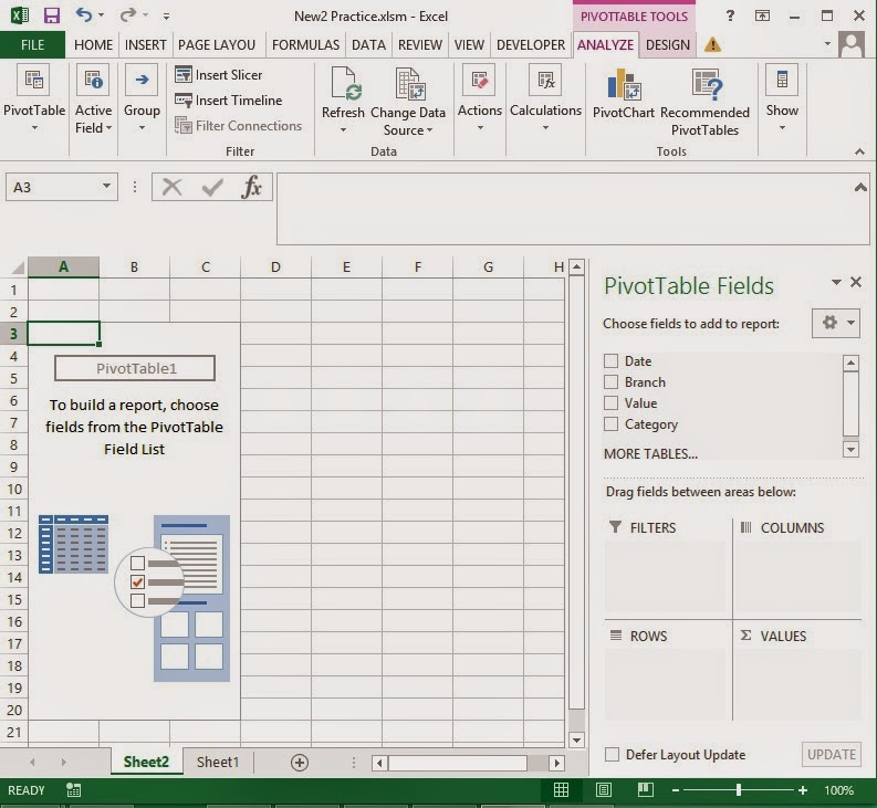

Above is the result I got. As you can see this method is little bit different to the quick pivot table creation method. Because in that method we got pivot table right away. In this method we have got a some kind of place holder for our pivot table. Actual pivot table will be created once we select the fields from the right side panel.  The bottom part of the right panel has separated to four areas. Filters, Columns, Rows and Values. Here you will notice that when you select text field or date field they will automatically listed under Rows area. And if you select a field which has numeric values it will automatically listed in the Value area. So now I will select Branch field and value field.
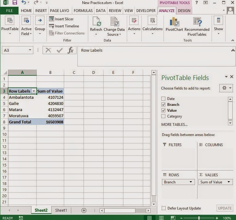

So now let's look at the Pivot table we have created. There are branches in the column A and Sum of values in column B. We can control the pivot table by the panel shown in the left hand side. You can see in that panel only check boxes of Branch and Value are checked. As a result only those two fields are shown in the pivot table. So let's click on the check box of the category field and see what will happen.


As you can see, now my pivot table has expanded. Now it shows both the Branch and Category. So in Rows area the category label is placed under Branch label. According to that, in the pivot table categories are listed under each branch. Think you need to list branches under each category. Then you can see how sales are varied for different branches for different categories. You can simply do this. what you need to do is drag Category label at the Rows area to top of the Branch label of same area. Here is the result you will get.


Now all the branches are listed under each category.So now let's move the category label to columns area and see what will happen.


Now it has also break down by categories as well. So each column represent a unique category. In addition to that you can filter column labels as you like. Not only that you can even pivot two fields. So let's interchange Branch and Category in the bottom part of the right panel and see what will happen.


So you can see how the Branches and Categories swapped with that action. This flexibility of the Excel pivot tables is a key reason to it's popularity.

Download a file from url using VBA

Sometimes our Excel VBA applications need to interact with websites. Downloading a file through a URL is a typical example. In this lesson you can learn how to do that using XMLHttpRequest and ADODB.Stream object. XMLHttp is used to request the data from the web server. Once we receive the data from the server, the ADODB.Stream object is used to write that data to a file. You can use this method to download file types such as image files, csv files etc.

So let’s start writing our macro to download a file using the Uniform Resource Locator (URL). Let’s name our Sub procedure as “DownloadFileFromURL”


Sub DownloadFileFromURL()

End Sub

First we need to declare a few variables.

Dim FileUrl As String
Dim objXmlHttpReq As Object
Dim objStream As Object

Next assign the URL of the file to the FileUrl variables

FileUrl = "URL of your file"

For an example if your file URL is https://www.example.com/images/chart.jpg then you can assign it to the variable as follows.

FileUrl = "https://www.example.com/images/chart.jpg"

Next step is to create a XMLHttp object to request the data from the server.

Set objXmlHttpReq = CreateObject("Microsoft.XMLHTTP")

Call the open method followed by the send method.

objXmlHttpReq.Open "GET", FileUrl, False, "username", "password"
objXmlHttpReq.send

Then check the status. If it equals 200 (OK), we can move to the next step.

If objXmlHttpReq.Status = 200 Then

Now we need to create an ADODB.Stream object to write the data(received) to a file.

Set objStream = CreateObject("ADODB.Stream")

Stream in programming means flow of data. In programming data is what flows between processors and input or output devices. Check this link to see all the Properties, Methods and Events of Stream object.

Stream Object Properties, Methods, and Events

But we need to use only a few of them here.

objStream.Open
objStream.Type = 1
objStream.Write objXmlHttpReq.responseBody
objStream.SaveToFile ThisWorkbook.Path & "\" & "file.jpg", 2
objStream.Close

In the SaveToFile method I have entered 2 as SaveOptions. So the program will overwrite the file with the data from the stream if the file already exists. If you don’t want to overwrite the existing file then replace it with 1.

objStream.SaveToFile ThisWorkbook.Path & "\" & "file.jpg", 1

Below is the full code which you can use to download a file through a URL.

Sub DownloadFileFromURL()

     Dim FileUrl As String
     Dim objXmlHttpReq As Object
     Dim objStream As Object

     FileUrl = "URL of your file"

     'example
     'FileUrl = "https://www.example.com/images/chart.jpg"

     Set objXmlHttpReq = CreateObject("Microsoft.XMLHTTP")
     objXmlHttpReq.Open "GET", FileUrl, False, "username", "password"
     objXmlHttpReq.send

     If objXmlHttpReq.Status = 200 Then
          Set objStream = CreateObject("ADODB.Stream")
          objStream.Open
          objStream.Type = 1
          objStream.Write objXmlHttpReq.responseBody
          objStream.SaveToFile ThisWorkbook.Path & "\" & "file.jpg", 2
          objStream.Close
     End If

End Sub

In the above example I showed how to download a .jpg file. But you can use this method to download other file types as well. Remember to change the file extension depending on the type of the file you download. For example if you are downloading a CSV file then the SaveToFile method should be changed as follows.

objStream.SaveToFile ThisWorkbook.Path & "\" & "file.jpg", 2

Contact Form

Name

Email *

Message *