How to Put Double Quotes in a String in VBA

In this lesson you will learn how to put double quotes in a string in Excel VBA. Sometimes your VBA application needs to output some text in an Excel sheet, in a form control or in the immediate window. For an example, assume you want to write Hello World! In cell A1 of the Sheet1. You can simply do it like this.

Sub WriteHelloWorldInSheet()

Worksheets("Sheet1").Range("A1").Value = "Hello World!"

End Sub

Or you can simply print this in the immediate window like this.

Sub PrintHelloWorldInImmediateWindow()

Debug.Print "Hello World!"

End Sub

But what if you want to output something like this in an Excel sheet or immediate window.,

"I admired both of them, especially Kevin," John said.

Excel VBA will give us a syntax error if we follow the above methods.

And if you try to output this in the immediate window, text will convert to a strange form like this.

So how do we put quotation marks in a string? There are two ways to solve this problem.

Method 1

Add an extra double quote in front of each quotation mark. So the quotation marks will be doubled. If you want to show two double quotes inside the string, then you will have to write four double quotes. I will explain this little more with our sample string.

As you can see there are two types of quotation marks in this image. Two red color double quotes and two green color double quotes. Red color quotes are ourter quotes. You don’t need to do anything with them. You have to double only the green color double quotes. So the final code should look like this.

Here is the complete subroutine.

Sub DoubleQuotesExample()

Worksheets("Sheet1").Range("A1").Value = """I admired both of them, especially Kevin,"" John said."

End Sub

You can use this same technique to print string in the immediate window as well.

Sub DoubleQuotesExampleImmediateWindow()

Debug.Print """I admired both of them, especially Kevin,"" John said."

End Sub

Next let’s look at how to use this method when there are consecutive double quotes.

Example - Output following in the cell A1 of the Sheet 1

"Apple""Mango""Orange"

So the rule of this method is, you have to add an extra double quote for each quotation mark. So the completed subroutine should look like this.

Sub ConsecutiveDoubleQuotes()

Worksheets("Sheet1").Range("A1").Value = """Apple""""Mango""""Orange"""

End Sub

Method 2

Use the ASCII code of the double quote. In this method you can use Chr(34) where you want the double quotes. So let’s consider our first example string again.

"I admired both of them, especially Kevin," John said.

We can replace the double quotes with Chr(34) like this.

Chr(34) & "I admired both of them, especially Kevin," & Chr(34) & " John said."

Remember to use ampersand(&) to concatenate text strings with Chr(34). Here is the completed subroutine to write that string to cell A1 of the Sheet1.

Sub DoubleQuotesExample_Method2()

Worksheets("Sheet1").Range("A1").Value = Chr(34) & "I admired both of them, especially Kevin," & Chr(34) & " John said."

End Sub

And here is how you can use this second method to print a string with double quotes in the immediate window.

Sub PrintDoubleQuotesImmediateWindow_Method2()

Debug.Print Chr(34) & "I admired both of them, especially Kevin," & Chr(34) & " John said."

End Sub

Next let’s look at how to use this method when there are consecutive double quotes in the strings. So let’s try to print the string below in the immediate windows using this second method.

"Apple""Mango""Orange"

The rule is, you need to replace " with Chr(34) and concatenate with ampersand(&). Therefore we can rewrite the above string like this.

Chr(34) & "Apple" Chr(34) & Chr(34) & "Mango" Chr(34) & Chr(34) & "Orange" & Chr(34)

Here is the completed subroutine

Sub ConsecutiveDoubleQuotes_Method2()

Debug.Print Chr(34) & "Apple"; Chr(34) & Chr(34) & "Mango"; Chr(34) & Chr(34) & "Orange" & Chr(34)

End Sub

You can also use these ASCII codes for various other characters. Check this page to see what characters you can print with ASCII codes.

ASCII Table

How to Add a Formula to a Cell Using VBA

In this lesson you can learn how to add a formula to a cell using vba. There are several ways to insert formulas to cells automatically. We can use properties like Formula, Value and FormulaR1C1 of the Range object. This post explains five different ways to add formulas to cells.

Table of contents
How to add formula to cell using VBA
Add formula to cell and fill down using VBA
Add sum formula to cell using VBA
How to add If formula to cell using VBA
Add formula to cell with quotes using VBA
Add Vlookup formula to cell using VBA

We use formulas to calculate various things in Excel. Sometimes you may need to enter the same formula to hundreds or thousands of rows or columns only changing the row numbers or columns. For an example let’s consider this sample Excel sheet.

In this Excel sheet I have added a very simple formula to the D2 cell.

=B2+C2

So what if we want to add similar formulas for all the rows in column D. So the D3 cell will have the formula as =B3+C3 and D4 will have the formula as =B4+D4 and so on. Luckily we don’t need to type the formulas manually in all rows. There is a much easier way to do this. First select the cell containing the formula. Then take the cursor to the bottom right corner of the cell. Mouse pointer will change to a + sign. Then left click and drag the mouse until the end of the rows.

However if you want to add the same formula again and again for lots of Excel sheets then you can use a VBA macro to speed up the process. First let’s look at how to add a formula to one cell using vba.

How to add formula to cell using VBA

Lets see how we can enter above simple formula(=B2+C2) to cell D2 using VBA

Method 1

In this method we are going to use the Formula property of the Range object.

Sub AddFormula_Method1()

     Dim WS As Worksheet

     Set WS = Worksheets("Sheet1")

     WS.Range("D2").Formula = "=B2+C2"

End Sub

Method 2

We can also use the Value property of the Range object to add a formula to a cell.

Sub AddFormula_Method2()

    Dim WS As Worksheet

    Set WS = Worksheets("Sheet1")

    WS.Range("D2").Value = "=B2+C2"

End Sub

Method 3

Next method is to use the FormulaR1C1 property of the Range object. There are few different ways to use FormulaR1C1 property. We can use absolute reference, relative reference or use both types of references inside the same formula.

In the absolute reference method cells are referred to using numbers. Excel sheets have numbers for each row. So you should think similarly for columns. So column A is number 1. Column B is number 2 etc. Then when writing the formula use R before the row number and C before the column number. So the cell A1 is referred to by R1C1. A2 is referred to by R2C1. B3 is referred to by R3C2 etc.

This is how you can use the absolute reference.

Sub AddFormula_Method3A()

    Dim WS As Worksheet

    Set WS = Worksheets("Sheet1")

    WS.Range("D2").FormulaR1C1 = "=R2C2+R2C3"

End Sub

If you use the absolute reference, the formula will be added like this.

If you use the manual drag method explained above to fill down other rows, then the same formula will be copied to all the rows.

In Majority cases this is not how you want to fill down the formula. However this won’t happen in the relative method. In the relative method, cells are given numbers relative to the cell where the formula is entered. You should use negative numbers when referring to the cells in upward direction or left. Also the numbers should be placed within the square brackets. And you can omit [0] when referring to cells on the same row or column. So you can use RC[-2] instead of R[0]C[-2]. The macro recorder also generates relative reference type code, if you enter a formula to a cell while enabling the macro recorder.

Below example shows how to put formula =B2+C2 in D2 cell using relative reference method.

Sub AddFormula_Method3B()

    Dim WS As Worksheet

    Set WS = Worksheets("Sheet1")

    WS.Range("D2").FormulaR1C1 = "=RC[-2]+RC[-1]"

End Sub

Now use the drag method to fill down all the rows.

You can see that the formulas are changed according to the row numbers.

Also you can use both relative and absolute references in the same formula. Here is a typical example where you need a formula with both reference types.

We can add the formula to calculate Total Amount like this.

Sub AddFormula_Method3C()

     Dim WS As Worksheet

     Set WS = Worksheets("Sheet2")

     WS.Range("C5").FormulaR1C1 = "=RC[-1]+RC[-1]*R2C2"

End Sub

In this formula we have a absolute reference after the * symbol. So when we fill down the formula using the drag method that part will remain the same for all the rows. Hence we will get correct results for all the rows.

Add formula to cell and fill down using VBA

So now you've learnt various methods to add a formula to a cell. Next let’s look at how to fill down the other rows with the added formula using VBA.

Assume we have to calculate cell D2 value using =B2+C2 formula and fill down up to 1000 rows. First let’s see how we can modify the first method to do this. Let’s name this subroutine as “AddFormula_Method1_1000Rows”

Sub AddFormula_Method1_1000Rows()

End Sub

Then we need an additional variable for the For Next statement

Dim WS As Worksheet
Dim i As Integer

Next, assign the worksheet to WS variable

Set WS = Worksheets("Sheet1")

Now we can add the For Next statement like this.

For i = 2 To 1000
     WS.Range("D" & i).Formula = "=B" & i & "+C" & i
Next i

Here I have used "D" & i instead of D2 and "=B" & i & "+C" & i instead of "=B2+C2". So the formula keeps changing like =B3+C3, =B4+C4, =B5+C5 etc. when iterated through the For Next loop.

Below is the full code of the subroutine.

Sub AddFormula_Method1_1000Rows()

     Dim WS As Worksheet
     Dim i As Integer

     Set WS = Worksheets("Sheet1")

     For i = 2 To 1000
         WS.Range("D" & i).Formula = "=B" & i & "+C" & i
     Next i

End Sub

So that’s how you can use VBA to add formulas to cells with variables.

Next example shows how to modify the absolute reference type of FormulaR1C1 method to add formulas upto 1000 rows.

Sub AddFormula_Method3A_1000Rows()

     Dim WS As Worksheet
     Dim i As Integer

     Set WS = Worksheets("Sheet1")

     For i = 2 To 1000
         WS.Range("D" & i).FormulaR1C1 = "=R" & i & "C2+R" & i & "C3"
     Next i

End Sub

You don’t need to do any change to the formula section when modifying the relative reference type of the FormulaR1C1 method.

Sub AddFormula_Method3B_1000Rows()

     Dim WS As Worksheet
     Dim i As Integer

     Set WS = Worksheets("Sheet1")

     For i = 2 To 1000
         WS.Range("D" & i).FormulaR1C1 = "=RC[-2]+RC[-1]"
     Next i

End Sub

Use similar techniques to modify other two types of subroutines to add formulas for multiple rows. Now you know how to add formulas to cells with a variable. Next let’s look at how to add formulas with some inbuilt functions using VBA.

How to add sum formula to a cell using VBA

Suppose we want the total of column D in the D16 cell. So this is the formula we need to create.

=SUM(D2:D15)

Now let’s see how to add this using VBA. Let’s name this subroutine as SumFormula.

Sub SumFormula()

End Sub

First let’s declare a few variables.

Dim WS As Worksheet
Dim StartingRow As Long
Dim EndingRow As Long

Assign the worksheet to the variable.

Set WS = Worksheets("Sheet3")

Assign the starting row and the ending row to relevant variables.

StartingRow = 2
EndingRow = 1

Then the final step is to create the formula with the above variables.

WS.Range("D16").Formula = "=SUM(D" & StartingRow & ":D" & EndingRow & ")"

Below is the full code to add the Sum formula using VBA.

Sub SumFormula()

     Dim WS As Worksheet
     Dim StartingRow As Long
     Dim EndingRow As Long

     Set WS = Worksheets("Sheet3")
     StartingRow = 2
     EndingRow = 15

     WS.Range("D16").Formula = "=SUM(D" & StartingRow & ":D" & EndingRow & ")"

End Sub

How to add If Formula to a cell using VBA

If function is a very popular inbuilt worksheet function available in Microsoft Excel. This function has 3 arguments. Two of them are optional.

Now let’s see how to add a If formula to a cell using VBA. Here is a typical example where we need a simple If function.

This is the results of students on an examination. Here we have names of students in column A and their marks in column B. Students should get “Pass” if he/she has marks equal or higher than 40. If marks are less than 40 then Excel should show the “Fail” in column C. We can simply obtain this result by adding an If function to column C. Below is the function we need in the C2 cell.

=IF(B2>=40,"Pass","Fail")

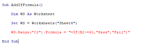
Now let’s look at how to add this If Formula to a C2 cell using VBA. Once you know how to add it then you can use the For Next statement to fill the rest of the rows like we did above. We discussed a few different ways to add formulas to a range object using VBA. For this particular example I’m going to use the Formula property of the Range object.

So now let’s see how we can develop this macro. Let’s name this subroutine as “AddIfFormula”

Sub AddIfFormula()

End Sub

However we can’t simply add this If formula using the Formula property like we did before. Because this If formula has quotes inside it. So if we try to add the formula to the cell with quotes, then we get a syntax error.

Add formula to cell with quotes

There are two ways to add the formula to a cell with quotes.

Method 1

Sub AddIfFormula_Method1()

     Dim WS As Worksheet

     Set WS = Worksheets("Sheet4")

     WS.Range("C2").Formula = "=IF(B2>=40,""Pass"",""Fail"")"

End Sub

Method 2

Sub AddIfFormula_Method2()

     Dim WS As Worksheet

     Set WS = Worksheets("Sheet4")

     WS.Range("C2").Formula = "=IF(B2>=40," & Chr(34) & "Pass" & Chr(34) & "," & Chr(34) & "Fail" & Chr(34) & ")"

End Sub

Add vlookup formula to cell using VBA

Finally I will show you how to add a vlookup formula to a cell using VBA. So I created a very simple example where we can use a Vlookup function. Assume we have this section in the Sheet5 of the same workbook.

So here when we change the name of the student in the C2 cell, his/her pass or fail status should automatically be shown in the C3 cell. If the original data(data we used in the above “If formula” example) is listed in the Sheet4 then we can write a Vlookup formula for the C3 cell like this.

=VLOOKUP(Sheet5!C2,Sheet4!A2:C200,3,FALSE)

We can use the Formula property of the Range object to add this Vlookup formula to the C3 using VBA.

Sub AddVlookupFormula()

     Dim WS As Worksheet

     Set WS = Worksheets("Sheet5")

     WS.Range("C3").Formula = "=VLOOKUP(Sheet5!C2,Sheet4!A2:C200,3,FALSE)"

End Sub

Swap Axis of an Excel Chart Without Changing Excel Sheet Data

This post explains how you can swap the axis of an Excel chart without swapping values in the sheet. Assume we have an Excel sheet like this.

If we select the data and insert a “Scatter with smooth lines” chart, then we will get a chart like this.

Or else we can insert a “Line” chart like this.

If you look at these charts, you can see that names are in the x axis. In the line chart names are visible in the x axis. But the Scatter chart shows some numbers instead of the names. Yet if you take the cursor to the Scatter chart it will show you the data points like this.

Therefore it is clear that the Scatter chart also has names in the x axis.

But then these charts don't make much sense according to how the Excel application has chosen the x axis. But it will be more understandable if we can set “Tests” as x axis instead of “Names”. One way to do that is re-arranging the data in the Excel sheet. However there is an easier way to do that without doing any change to the Excel data. We can simply do that by changing the x axis of the chart. Below are the steps to change the x axis.

First click somewhere on the chart. You will see two new tabs appear at the Excel ribbon called “Design” and “Format”.

Go to the design tab and click on the “Switch Row/Column” icon in the “Data” Group.

Scatter chart will change to something like this.

You can do the same for the line chart as well.

How to Add Search Function to a VBA Data Entry Application

In this post I will show you how to add a search function to a data entry application. I have already created the data entry form and sheet to save the data.

This is the form used to input the data.

Entered data will be saved to this worksheet.

Now the next step is to add the search function to this application. There are two ways to do that. We can either add the search function to existing data input form or add the search function to a dedicated form. So in this example I’m going to add the search function to a separate form. After creating the two forms you can add buttons to switch between each form. Here is the search form designed for this application. Labels and textboxes are the same as input form. I have changed the title to “SEARCH ORDER INFORMATION”. Also the “ENTER” button is replaced by the “SEARCH” button. Name of the “SEARCH” button is “cmdSearch''.

In this application, users will be able to search the information using the order number. So the user will enter the order number they want to search and click on the search button. Then the program will check the data sheet and show the relevant information in the form.

Now let’s develop the code for the “SEARCH” button.

First we need to declare a few variables

Dim WS_Data As Worksheet
Dim LastRow As Long
Dim i As Long
Dim SearchedValue As String
Dim DataArr() As Variant

Then assign the worksheet for the WS_Data variable.

Set WS_Data = Worksheets("Data")

Next find the last row of the Data sheet.

LastRow = WS_Data.Cells.Find("*", [A1], , , xlByRows, xlPrevious).Row

Now we need to find the matching row from the data sheet and show that information in the form. There are various ways to find the matching row from the data sheet. This post explains three different ways to find the matching row.

Get Row Number of a Matching Value

So I’m going to use the method 2 explained in that post. In this method we use an array to hold all the data in the worksheet. Using an array will increase the speed of the searching process if you have a large amount of data.

Add all the data from Data sheet to an array.

DataArr = WS.Range("A1:G" & LastRow)

Name of the “Order Number” textbox is txtOrderNumber. So we can assign the value to the SearchedValue variable from the Order Number textbox like this.

SearchedValue = txtOrderNumber.Value

Before proceeding further we need to check whether the user has entered a value to the Order Information textbox.

If Len(SearchedValue) > 0 Then

End If

Above If statement will be true if there is a value in the textbox.

Then we can use a For Next statement to loop through the data of the array.

If Len(SearchedValue) > 0 Then
     For i = 1 To UBound(DataArr, 1)

     Next i
End If

Check for the matching value using StrComp function

If Len(SearchedValue) > 0 Then
     For i = 1 To UBound(DataArr, 1)
          If StrComp(DataArr(i, 1), SearchedValue, vbTextCompare) = 0 Then

          End If
     Next i
End If

If a match is found then write information from that row to textboxes and exit the for loop.

If Len(SearchedValue) > 0 Then
     For i = 1 To UBound(DataArr, 1)
          If StrComp(DataArr(i, 1), SearchedValue, vbTextCompare) = 0 Then
               txtSize.Value = DataArr(i, 2)
               txtSerialNumber.Value = DataArr(i, 3)
               txtProjectNumber.Value = DataArr(i, 4)
               txtType.Value = DataArr(i, 5)
               txtDate.Value = DataArr(i, 6)
               txtSurveyor.Value = DataArr(i, 7)
               Exit For
          End If
     Next i
End If

So the complete code of the “SEARCH” button should look like this.

Private Sub cmdSearch_Click()

Dim WS_Data As Worksheet
Dim LastRow As Long
Dim i As Long
Dim SearchedValue As String
Dim DataArr() As Variant

Set WS_Data = Worksheets("Data")

LastRow = WS_Data.Cells.Find("*", [A1], , , xlByRows, xlPrevious).Row
DataArr = WS_Data.Range("A1:G" & LastRow)
SearchedValue = txtOrderNumber.Value

If Len(SearchedValue) > 0 Then
     For i = 1 To UBound(DataArr, 1)
          If StrComp(DataArr(i, 1), SearchedValue, vbTextCompare) = 0 Then
               txtSize.Value = DataArr(i, 2)
               txtSerialNumber.Value = DataArr(i, 3)
               txtProjectNumber.Value = DataArr(i, 4)
               txtType.Value = DataArr(i, 5)
               txtDate.Value = DataArr(i, 6)
               txtSurveyor.Value = DataArr(i, 7)
               Exit For
          End If
     Next i
End If

End Sub

Assume a user enters 8782 and performs a search.

Then the program will show the result in the form like this.

Create a Masked Password Using VBA

In this lesson you will learn how to create a masked password using VBA. Masked passwords are essential for the security of the data of the user. Because if you enter a password to an unmasked textbox or inputbox then the password will be visible to others around you. But if you use a masked textbox or inputbox then Excel will hide the password with asterisks.

Here is a custom VBA form designed to get the password from a user.

But as the textbox is not masked, the password entered will be visible.

So now let’s look at how to mask a password in Excel VBA forms.

First, open the visual basic editor. You can use “Developer” tab or the keyboard shortcut Alt + F11

Can’t see the developer tab in your Excel application? Learn how to show the Developer tab

Next, select the textbox you want to apply the mask to.

Go to the properties window and find “PasswordChar” field

Now select the character you want to show when the user types password. The asterisk(*) is the typical symbol used for this.

All set with the form. Now asterisks will be displayed when you enter characters in the textbox.

Retrieve password from the textbox

Now you learnt how to hide passwords with asterisks in Excel VBA textboxes. But do you know how to retrieve the password entered by the user? You can use the below code to print the password in the immediate window. cmdOK is the name of the OK button used in the form.

Private Sub cmdOk_Click()

     Dim Pwd As String

     Pwd = frmPwd.TextBox1.Value
     Debug.Print Pwd

End Sub

Now when the user clicks the OK button after entering the password, the program will assign that to the variable Pwd of type string. Then you can use that variable for the next steps such as password validation or password matching.

Hide password with asterisks in an inputbox

You can use inputbox to get input from users. But is it possible to mask a password with asterisks in an inputbox? Unfortunately you can’t use the above method for an inputbox. But this page explains how to use a private InputBox to mask the password with asterisks.

Private InputBox to mask the password with asterisks

Get Row Number of a Matching Value

In this lesson you can learn how to find the row number of a matching value. This page explains about 3 ways to do this. You can adapt a solution according to your preference. These techniques will be very helpful when you develop applications like data entry systems. Because in these types of applications you may need to show the matching result to the user. For example you might want to let the user search with a text using a textbox or a inputbox.

I will use this sample worksheet to explain these three methods.

Suppose user search for the code “C00KLCMU14”. So the program should return the matching row number as 14.

Method 1

'Row number of matching value
Sub MatchingRowNumber()

Dim WS As Worksheet
Dim MatchingRow As Long
Dim i As Long
Dim SearchedValue As String

Set WS = Worksheets("Sheet1")

SearchedValue = "C00KLCMU14"

For i = 1 To 10000
     If StrComp(WS.Range("B" & i).Value, SearchedValue, vbTextCompare) = 0 Then
          MatchingRow = i
          Exit For
     End If
Next i

MsgBox MatchingRow

End Sub

In the above macro the For Next loop is used assuming there are 10,000 rows of data. But if you have data up to x rows then you should replace For i = 1 to 10000 with For i = 1 to x

If no match is found, the message box will output 0 because zero is the default value of the Long data type.

However there is one problem with this solution. It is that if you have data in a higher number of rows in your Excel sheet then the program will take considerable time to output the result. But we can avoid this problem if we use arrays.

Method 2

Assume we have one million rows of data in our sheet. Here is how you can use an array to get the required result without delay.

Sub MatchingRowNumber_ArraySolution()

Dim WS As Worksheet
Dim MatchingRow As Long
Dim i As Long
Dim SearchedValue As String
Dim DataArr() As Variant

Set WS = Worksheets("Sheet1")

DataArr = WS.Range("A1:E1000000")
SearchedValue = "C00KLCMU14"

For i = 1 To 1000000
     If StrComp(DataArr(i, 2), SearchedValue, vbTextCompare) = 0 Then
          MatchingRow = i
         Exit For
     End If
Next i

MsgBox MatchingRow

End Sub

This is an easy way to write a range to an array.

DataArr = WS.Range("A1:E1000000")

Things you need to remember when creating an array using the above method.

• This method always creates a multidimensional array.
• Indexes of both dimensions will start from 1.

Want to learn more about arrays? Check these lessons.

Multidimensional Arrays in VBA
Quick Multidimensional Array from Excel Range
Quickly Write Multidimensional Array to Excel Range

So far we have discussed two methods of finding the row number of a matching value. But sometimes cells can contain spaces before or after the values. So if there are spaces like that, then the program will not be able to find the matching value. To avoid this issue we can use the Trim function to remove unwanted spaces before or after the values.

This is how you can use the Trim function for the first method.

Replace

If StrComp(WS.Range("B" & i).Value, SearchedValue, vbTextCompare) = 0 Then

With

If StrComp(Trim(WS.Range("B" & i).Value), SearchedValue, vbTextCompare) = 0 Then

And here is how you can use the Trim function for the second method.

Replace

If StrComp(DataArr(i, 2), SearchedValue, vbTextCompare) = 0 Then

With

If StrComp(Trim(DataArr(i, 2)), SearchedValue, vbTextCompare) = 0 Then

Also if you get the SearchedValue from the user from a method such as input box or textbox then you can use the Trim function to remove unwanted spaces from SearchedValue as well.

If StrComp(Trim(DataArr(i, 2)), Trim(SearchedValue), vbTextCompare) = 0 Then

Method 3

Now let’s look at the third method to find the row number of a matching value. You can use the Find method to return the row number of the matching value.

Sub MatchingRowNumber_FindFunction()

Dim WS As Worksheet
Dim MatchingRow As Long
Dim SearchedValue As String

Set WS = Worksheets("Sheet1")
SearchedValue = "C00KLCMU14"
MatchingRow = WS.Cells.Find(What:=SearchedValue, After:=Cells(1, 1), LookIn:=xlFormulas, _
     LookAt:=xlWhole, SearchOrder:=xlByRows, SearchDirection:=xlNext, _
     MatchCase:=False, SearchFormat:=False).Row

MsgBox MatchingRow
End Sub

This will output the correct row number if there is a match. However if there is no match then the program will throw an error.

To avoid this error, we can use the error handling technique as follows. So if there is no match, the program will output 0.

Sub MatchingRowNumber_FindFunction()

Dim WS As Worksheet
Dim MatchingRow As Long
Dim SearchedValue As String

Set WS = Worksheets("Sheet1")
SearchedValue = "C00KLCMU14"

On Error Resume Next
MatchingRow = WS.Cells.Find(What:=SearchedValue, After:=Cells(1, 1), LookIn:=xlFormulas, _
     LookAt:=xlWhole, SearchOrder:=xlByRows, SearchDirection:=xlNext, _
     MatchCase:=False, SearchFormat:=False).Row
If Err.Number <> 0 Then
     If Err.Number = 91 Then
         MatchingRow = 0
     Else
         MsgBox "Unknown Error"
         On Error GoTo 0
         Exit Sub
     End If
End If
On Error GoTo 0

MsgBox MatchingRow
End Sub

However this method will not work if cells contain extra spaces before or after the values.

Access Formula Bar Using Keyboard - Excel 2013

In the last post we discussed how to activate the edit mode for the active cell using a keyboard shortcut. From this post you can learn how to access the formula bar in Excel 2013 using the keyboard. Here are the steps to follow.

Click on the “File” menu.

Then click on the “Options”

Go to “Advanced” tab and remove tick from the “Allow editing directly in cells”

Now the cursor will jump to the formula bar when you press F2 on the keyboard.