Want to become an expert in VBA? So this is the right place for you. This blog mainly focus on teaching how to apply Visual Basic for Microsoft Excel. So improve the functionality of your excel workbooks with the aid of this blog. Also ask any questions you have regarding MS Excel and applying VBA. We are happy to assist you.

How to Remove the Last Full Stop from Every Cell in a Selection Using VBA

In today's post, I'm going to show you how to remove the last full stop from a cell in Excel using VBA. This can be especially useful when cleaning up text data. For example, if you have a list of sentences and you want to ensure that none of them end with a full stop, you can use this simple VBA code.

Let’s consider this example worksheet.

Sample sentences with full stop marks

Here's the complete code:

Sub RemoveLastFullStop()

Dim MyCell As Range
Dim trimmedSentence As String
Dim LastChar As String

For Each MyCell In Selection

    If MyCell.Value <> "" Then
    
        MyCell.Value = Trim(MyCell.Value)
        
        trimmedSentence = MyCell.Value
        
        LastChar = Right(trimmedSentence, 1)
        
        If StrComp(LastChar, Chr(46), vbBinaryCompare) = 0 Then
            MyCell.Value = Mid(trimmedSentence, 1, Len(trimmedSentence) - 1)
        End If
    End If
    
Next

MsgBox "Completed!", vbInformation, ""

End Sub

Below is the explanation of the above code.

Loop Through Each Cell in the Selection.
The code starts by looping through each cell in the selected range.

For Each MyCell In Selection

Check if the Cell is Not Empty.
Inside the loop, we check if the cell is not empty.

If MyCell.Value <> "" Then

Trim the Cell Value
We then use the Trim function to remove any leading or trailing spaces from the cell value.

MyCell.Value = Trim(MyCell.Value)

Get the Last Character
Next, we store the trimmed sentence in a variable and get the last character of the sentence.

trimmedSentence = MyCell.Value
LastChar = Right(trimmedSentence, 1)

Check if the Last Character is a Full Stop
We then check if the last character is a full stop using the StrComp function.

If StrComp(LastChar, Chr(46), vbBinaryCompare) = 0 Then

Here Chr(46) is used to represent the full stop (.) character.

This is the breakdown of what Chr(46) does:

Chr: This function returns the character associated with the specified character code.
46: This is the ASCII code for the full stop (.) character.
So, Chr(46) converts the ASCII code 46 into the corresponding character, which is a full stop.

If it is a full stop, we remove it by taking all characters except the last one.

MyCell.Value = Mid(trimmedSentence, 1, Len(trimmedSentence) - 1)

Display a Message Box

After the loop is done, we display a message box to indicate that the process is complete.

MsgBox "Completed!", vbInformation, ""

By following these steps, you can easily remove the last full stop from each cell in your selected range. This is the result you will get when run the above macro

Result after removing full stops.

Select Method of Range Class Failed Error in VBA

In the Excel VBA development, encountering errors can be a common yet frustrating experience. A frequent issue that specially new developers encounter is the "Select Method of Range Class Failed" error. This article aims to unveil this error, offering insights into its cause and presenting a solution to resolve it.


Understanding the "Select Method of Range Class Failed" Error

The "Select Method of Range Class Failed" error typically arises when VBA code attempts to select a range that is inaccessible at the time of the code execution.

Cause of the "Select Method of Range Class Failed" Error

Understanding the underlying cause is critical to resolving the error. Below is the reason for this error.

Inactive Worksheet
Trying to select a range on a worksheet that is not currently active can lead to this error. Let’s consider this example Excel workbook.

Example workbook

This Excel file contains two worksheets. “Input” and “Output” sheets. Currently we are in the “Input” sheet. So the “Input” sheet is the worksheet active at the moment. Assume we tried to select the A1 cell of the “Output” now using the below subroutine.

Sub InactiveWorksheetExample()

Dim WS_Input As Worksheet
Dim WS_Output As Worksheet

Set WS_Input = Worksheets("Input")
Set WS_Output = Worksheets("Output")

WS_Output.Range("A1").Select

End Sub

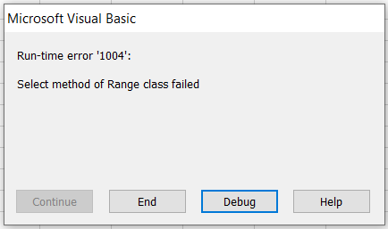
Here what we are doing is we are asking the macro to select a cell from a worksheet which is not active. So this will throw the following error - Run-time error '1004' - Select method of Range class failed.

Select Method of Range Class Failed Error


How to Fix the Error

To tackle this error, we can simply activate the required sheet. So before selecting a range, make sure the relevant sheet is activated using Worksheet.Activate method. Here is how you can modify the above subroutine to do that.

Sub InactiveWorksheetExample()

Dim WS_Input As Worksheet
Dim WS_Output As Worksheet

Set WS_Input = Worksheets("Input")
Set WS_Output = Worksheets("Output")

WS_Output.Activate
WS_Output.Range("A1").Select

End Sub

Method 'Range' of object '_Worksheet' Failed Error in VBA

When working with VBA in Excel, encountering errors is not uncommon, especially when dealing with range objects. One such error is the "Method 'Range' of object '_Worksheet' failed". In this post we will explore the causes of this VBA error and how to effectively troubleshoot and resolve it.


Introduction to Method 'Range' of object '_Worksheet' Failed Error

The "Method 'Range' of object '_Worksheet' failed" error in VBA typically occurs when the code tries to reference a range that does not exist or is incorrectly specified. This error can be frustrating, especially for those new to VBA. Understanding the nature of this error is the first step in resolving it.

Common Causes of the Range Method Error

Incorrect Range Reference
When the specified range in the code does not exist in the worksheet. Here is a simple example.

Sub SelectRange()

   Dim WS As Worksheet

   Set WS = ActiveSheet

   WS.Range("B1400000").Select

End Sub

In this example, macro is trying to select a cell called B1400000. But such a cell is not available in Excel because the row limit of the Excel application is 1,048,576.

Check this post to see more details about Excel row limit.
Number of rows in Excel

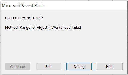
So when we run the macro it will show this error message.

Method 'Range' of object '_Worksheet' Failed Error

Troubleshooting the Range Method Error

To troubleshoot this error, follow these steps.

Check Range References
Ensure that the range referenced in the code exists in the worksheet.

Debugging
Use VBA's debugging tools, like the Immediate Window and Local Window, to track the values and state of variables at runtime. If your code is referencing dynamic ranges then you can detect whether it is referencing nonexistent ranges.

Error Handling
Implement error-handling routines to catch and handle errors.

The error "Method 'Range' of object '_Worksheet' failed" can be a hurdle in VBA programming, but with careful examination of the code, validation of references, and implementation of best practices, it can be effectively managed and resolved. Understanding the root causes and having a structured approach to troubleshooting are key to overcoming this challenge in Excel VBA.

How to Get Selected Item from VBA Listbox

In this lesson, we will explore how to extract the selected value from a multicolumn listbox using VBA in Excel. This is particularly useful when you have a listbox filled with multiple columns of data and you need to retrieve specific values based on user interaction. The process may seem complex, but with the right approach, it becomes a straightforward task.

Before diving into extracting values, it's crucial to understand what a listbox is. Essentially, it's a VBA control that can display items across multiple columns, like a simple table or spreadsheet. This functionality is very useful when you need to show more than one attribute of an item in a VBA control. Because in other VBA controls such as text boxes you can only show one attribute. So the VBA listboxes enhance the user experience by allowing users to view and select from a range of related data points.

Now let’s look at how we can get selected items from a VBA listbox in a few different ways.

Sample Excel sheet to demonstrate how to get selected item from a listbox

Above is a sample dataset consisting of twenty data entries. This dataset includes various fields such as Medicine ID, Medicine Name, Unit, Price, Supplier Name, Address, Phone, Rating and Supply Time. Please note that this data is entirely fictional and created for example purposes only.

Understanding the Listbox Properties
Before diving into the code, it’s important to understand two crucial properties of the listbox: List and ListIndex. The List property represents the array of items in the listbox, while ListIndex refers to the index of the selected item.

The primary challenge in working with multicolumn listboxes is retrieving the user’s selection, particularly when the listbox contains several columns. Let’s consider this example user form.

Sample VBA Listbox

User has entered a value in the supplier name field and hit the search button. Now all the data related to that supplier name is shown in the listbox. Assume the name of the form is afrmViewDat and name of the listbox is lstSearchResult.

Using the ListIndex Property

The ListIndex property of a listbox is your starting point. The ListIndex property of a listbox returns the index of the selected item. However, it's important to remember that the index starts at 0. Here’s how you can use it.

Sub GetListIndex()

   Dim selectedIndex As Integer

   With frmViewData.lstSearchResult
     selectedIndex = .ListIndex
   End With

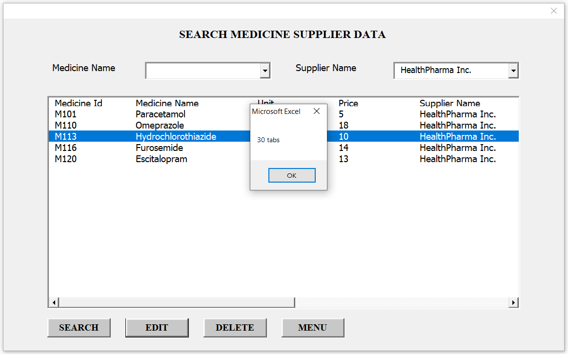
   MsgBox selectedIndex

End Sub

So here is the result of the above subroutine.

Listindex property returns index of the selected item

This method is straightforward but only works well when single selection is enabled. Because if multiselect is on and if the user has selected multiple items, then this subroutine will only return the index of the item you selected lastly.

What will happen if the user doesn’t select any item? Then -1 will be returned as the result. So we can use this value to check whether the user has selected any item before executing the rest of the code.

-1 is returned when no item is selected

Extracting Value from a Specific Column of the Selected Row - Using List Property

Once you have the row number, you can extract the value from a specific column using the List property. The List property can take two parameters: row index and column index. For instance, if you want to get the value from the second column of the selected row, you can use this approach.

Sub GetSelectedValue_Method1()

   Dim selectedIndex As Integer
   Dim selectedValue As String

   With frmViewData.lstSearchResult
     selectedIndex = .ListIndex
     If selectedIndex <> -1 Then
       selectedValue = .List(selectedIndex, 1) ' 1 for the second column
     Else
       selectedValue = "No selection"
     End If
   End With

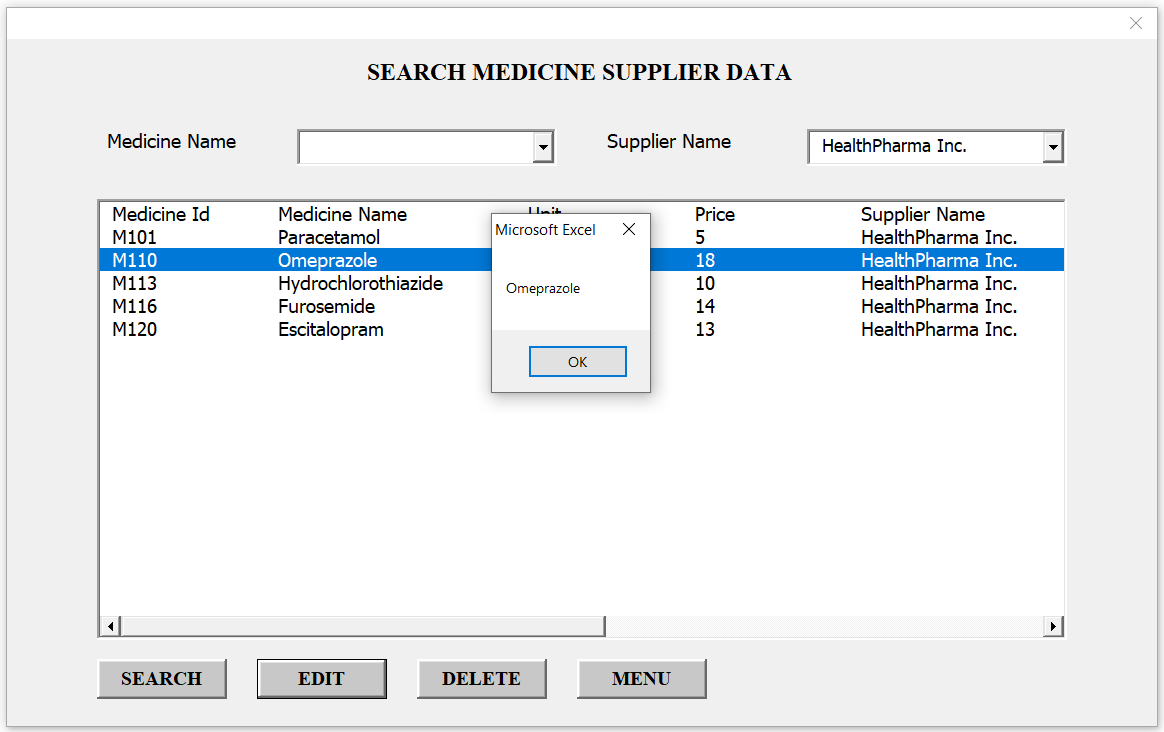
   MsgBox selectedValue

End Sub
Get value of a particular column of the selected row of the listbox

Handling Multiple Selections For MultiSelect Enabled ListBoxes

Things get a bit trickier when dealing with listboxes which are set to allow multiple selections. In such cases, you’ll need to iterate through each item in the listbox, checking if it’s selected and then retrieving the required column values. Below subroutine will get values of the second column for all the selected rows.

Sub GetSelectedValues_ForMultiselect()

   Dim i As Integer
   Dim selectedValues As String

   With frmViewData.lstSearchResult
     For i = 0 To .ListCount - 1
       If .Selected(i) Then
         selectedValues = selectedValues & .List(i, 1) & "; "
       End If
     Next i
   End With

   MsgBox selectedValues

End Sub
Get values of a particular column for all the selected rows of a listbox

Extracting Selected Value from a Listbox - Using Column Property

In the above examples, we learnt how to get a selected value using Listindex and List properties. However you can also use the Listindex with Column property to get the selected values from a listbox. Below example subroutine shows how you can get the column 3 value of the selected row.

Sub GetSelectedValue_Method2()

   Dim selectedValue As String

   With frmViewData.lstSearchResult
     If .ListIndex <> -1 Then
       selectedValue = .Column(2, .ListIndex) '2 for the third column
     Else
       selectedValue = "No selection"
     End If
   End With

   MsgBox selectedValue

End Sub
Get selected value of a listbox using Listindex and column properties

Tips and Tricks for Effective Coding

Remember that VBA is zero-indexed: The first column is column 0, the second is column 1, and so on. Same for the rows.
Always check if an item is selected in the listbox to avoid runtime errors.
Use meaningful variable names for clarity and maintenance purposes.

Also read
Populate Userform Listbox from Range
Add Horizontal Scrollbar to a Listbox
Fill a Listbox From an Array

Add Single Quotes to Excel Cells Using VBA

In our previous post we learnt the uses of adding single quotes to the beginning of cells.

Uses of Adding Single Quotes to Start of Excel Cells

In this lesson you will learn how to add single quotes to Excel cells using VBA. First of all, let’s see how we can do this manually in Excel. Because Excel shows unusual behavior when you add a single quote at the beginning of a cell.

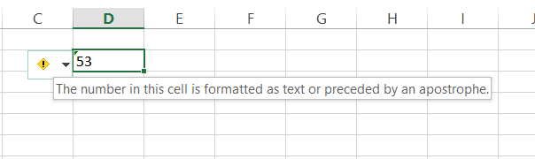
Assume you want to add ‘53 to an Excel cell. Then when you enter '53 to an Excel cell it will show only 53 with a small green triangle at the upper left corner of the cell.

When added single quote before a number in a cell

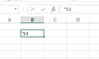
But in the formula bar you can still see the single quote before the number.

Formula bar still show the single quote before the number

Also when you select the cell a small icon will appear and if you take your cursor on top of it, you will see this kind of message.

Message

Then what if we want to see a single quote at the beginning of the cell. Solution is simple. You need to add two single quotes.

Add two single quotes

Here one single quote is shown in the cell. However you can see both single quotes in the formula bar.

Assume you want to add single quotes at both left and right of the content of the cell.
Example - '53'
How can we do that? To do this you need to add two single quotes at the beginning and only one single quote at the end like this.
''53'

Add single quotes at both sides of the cell content

Now let’s see how we can add single quotes to Excel cells using VBA. When we automate this in VBA we need to consider the above behavior too.
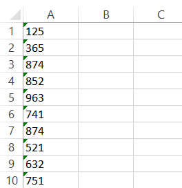
Let’s consider this sample Excel sheet.

Sample Excel sheet

Sheet has 10 values in column A. Assume we want to add a single quote in front of each value. There are two ways to do this in VBA. We can use either ASCII code or we can use single quotes inside double quotes. First let’s see how we can do this using ASCII code. Assume the name of the worksheet is “My Data”.

Method 1 - Using ASCII code

Sub Add_Single_Quote()

   Dim WS As Worksheet
   Dim i As Integer

   Set WS = Worksheets("My Data")

   For i = 1 To 10
     WS.Range("A" & i).Value = Chr(39) & WS.Range("A" & i).Value
   Next i

End Sub

In the above code Chr(39) represents the single quote character. Here you can find the full list of ASCII codes.

ASCII Table

Also a For loop is used to iterate through each value in column A.

Method 2 - Using Single quotes directly inside double quotes

Sub Add_Single_Quote_Method2()

   Dim WS As Worksheet
   Dim i As Integer

   Set WS = Worksheets("My Data")

   For i = 1 To 10
     WS.Range("A" & i).Value = "'" & WS.Range("A" & i).Value
   Next i

End Sub

Below is the result we get when we run any of the above subroutines.

Single quote is not shown in the result

Like in the manual scenario, we only get a green triangle at the upper left corner instead of the single quote. To show a single quote we need to add two single quotes using VBA. For that we can modify the above two macro as follows.

Method 1

Sub Add_Single_Quote()

   Dim WS As Worksheet
   Dim i As Integer

   Set WS = Worksheets("My Data")

   For i = 1 To 10
     WS.Range("A" & i).Value = Chr(39) & Chr(39) & WS.Range("A" & i).Value
   Next i

End Sub

Method 2

Sub Add_Single_Quote_Method2()

   Dim WS As Worksheet
   Dim i As Integer

   Set WS = Worksheets("My Data")

   For i = 1 To 10
     WS.Range("A" & i).Value = "''" & WS.Range("A" & i).Value
   Next i

End Sub

Now we will see a single quote before each value as expected.

Single quotes is added in front of each value

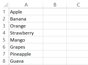
Next let’s see how we can add a single quote at both sides of the cell content. Let’s consider this new sheet. Assume the name of the sheet is “Fruits”.

New example worksheet

Below are the two methods to add single quotes at either side of the fruit names.

Method 1

Sub Add_Single_Quotes_At_Both_Sides()

   Dim WS As Worksheet
   Dim i As Integer

   Set WS = Worksheets("Fruits")

   For i = 1 To 8
     WS.Range("A" & i).Value = Chr(39) & Chr(39) & WS.Range("A" & i).Value & Chr(39)
   Next i

End Sub

Method 2

Sub Add_Single_Quotes_At_Both_Sides_Method2()

   Dim WS As Worksheet
   Dim i As Integer

   Set WS = Worksheets("Fruits")

   For i = 1 To 8
     WS.Range("A" & i).Value = "''" & WS.Range("A" & i).Value & "'"
   Next i

End Sub

You will get this result if you run any of the above macros.

Single quotes added at both sides of the cell content

Uses of Adding Single Quotes to Start of Excel Cells

Adding single quotes to the start of cells in Excel can be necessary in various scenarios to ensure data accuracy and proper interpretation. Here are a few scenarios where this technique might be useful.

Preserving Leading Zeros

When dealing with numeric codes or identifiers that begin with zeros, Excel might automatically remove leading zeros. Adding a single quote before such values prevents Excel from treating them as numbers, preserving the leading zeros.
Example:
00123 might become 123
'00123 remains as is

Preserving leading zeros using single quotes

Preparing Data for SQL Queries

In SQL queries, single quotes are often used to denote string values. If you are creating SQL queries in Excel and have a list of values, adding single quotes ensures that they are recognized as strings.
Example:
Apple might become 'Apple'

SQL query example

Handling Special Characters

If your data contains special characters that might have specific meanings in Excel or other applications, adding single quotes can help avoid misinterpretation.
Example:
=SUM(A1:A10) might be seen as a formula
'=SUM(A1:A10) ensures it's treated as text

Show formulas using single quotes

Creating CSV Files

When creating Comma-Separated Values (CSV) files, adding single quotes to cells can be beneficial. It helps maintain the intended format, especially when dealing with leading zeros or text that might resemble numerical data.
Example:
01234, 56789 might become 1234, 56789
'01234, 56789 remains as is

Also read
Add Single Quotes to Excel Cells Using VBA
How To Quote All Cells Of A CSV File
How to Put Double Quotes in a String in VBA

Extract Formulas From Cells Using VBA

In Excel, formulas are the backbone of data analysis and calculations. Extracting these formulas using VBA can be a powerful tool for various purposes. In this guide, we'll explore step by step how to use VBA to extract formulas from cells.

Here are a few scenarios where we need to extract formulas from cells using vba

  • To help in keeping track of changes made to formulas over time.
  • Analyze formulas to identify potential errors or inconsistencies.
  • Extracting formulas can help you analyze dependencies and relationships between different cells.
  • To partially automate the documentation process, providing insights of the logic behind calculations.

Now let’s see how we can develop a macro to extract a formula from a cell using VBA. First let’s see how we can get the formula from a particular cell we want. Let’s consider this example sheet.

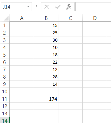
Sample worksheet with one formula

This worksheet has some values from B1 cell to B9 cell. Then I have put the following formula in cell B11.
=SUM(B1:B9)

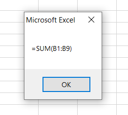
Assume the name of the worksheet is “Sheet1”. Then the following subroutine will show the formula of cell B11 in a message box.

Sub ExtractOneFormula()

   Dim WS As Worksheet

   Set WS = Worksheets("Sheet1")

   MsgBox WS.Range("B11").Formula

End Sub
Macro will extract and show the formula in a message box

Now we learnt how to get a formula from a particular cell using VBA. Next let’s look at how to get a list of all the formulas in a sheet with cell addresses. Let’s consider this example Excel sheet.

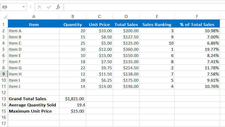
Sample Excel sheet with lots of formulas

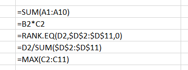
In this worksheet, Total sales in column D is calculated using formulas. For an example D2 cell has following formula
=B2*C2

Then Sales Ranking in column E is also calculated using formulas. For an example E2 cell has the following formula.
=RANK.EQ(D2,$D$2:$D$11,0)

Also % of Total Sales in column F is calculated using formulas. F2 cell has following formula
=D2/SUM($D$2:$D$11)

Then 3 fields(Grand Total Sales, Average Quantity Sold, Maximum Unit Price) in cells B13, B14 and B15 are calculated using following formulas.

Grand Total Sales =SUM(D2:D11)
Average Quantity Sold =AVERAGE(B2:B11)
Maximum Unit Price=MAX(C2:C11)

Then here is the macro to print all the formulas and their cell addresses in the immediate window

Sub ExtractFormulas()

   Dim WS As Worksheet
   Dim Rng As Range

   Set WS = Worksheets("Sheet2")

   For Each Rng In WS.UsedRange
     If Rng.HasFormula = True Then
       Debug.Print "Formula in " & Rng.Address & ": " & Rng.Formula
     End If
   Next Rng

End Sub
All the formulas are extracted and printed in the immediate window

In the above subroutine, the statement “If Rng.HasFormula = True Then” is used to identify the cells having formulas.

Also Rng.Address statement outputs the cell address of the cell and Rng.Formula statement output formula of that cell.

Also read
How to Add a Formula to a Cell Using VBA
Access Formula Bar Using Keyboard

Contact Form

Name

Email *

Message *