How to Clear the Immediate Window Using VBA

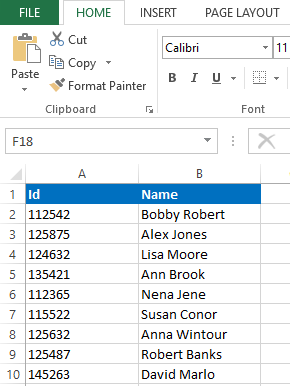
A VBA program can have multiple subroutines and functions. If you are a programmer you will need to test these subroutines and functions while developing the VBA code. Then the immediate window is a helpful tool you can use to test your components. If it is a subroutine, then you can print your variables using debug.print method to ensure whether they are calculated correctly. If it is a function you can print the return value in the immediate window.

From one of our previous posts we learnt how to output data in VBA using a few different ways. In that post you can find how to output data to Immediate window using VBA.

Output data in Excel VBA

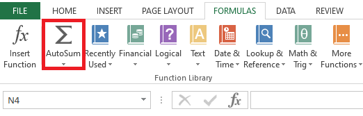
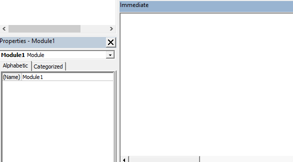
So today I'm going to show you how to clear the immediate window automatically using VBA. You may know how to clear it manually. If you don't know, follow these simple steps. First select everything in the immediate window. Then press the delete key on the keyboard to delete everything. If the immediate window is not visible you can use shortcut keys “Ctrl + G” to view the immediate window. Also if the cursor is in a different window than the immediate window, and if you press the above shortcut keys, then the cursor will move to the immediate window giving you access to the immediate window.

Now let’s look at how we can clear the immediate window using VBA. We can use the Application.Sendkeys method to clear the immediate window using VBA. Application.Sendkeys method lets us send keystrokes to the active application. So here is the order of keystrokes we need to send to clear the immediate window.

Ctrl + G
Ctrl + A
Delete

Ctrl + G will activate the immediate window. Then Ctrl + A will select everything in the immediate window. And Delete keystroke will delete the content from the immediate window. However in the Application.Sendkeys method, these keys are represented by one or more characters. Ctrl is represented by ^ character. You can simply use g and a keys to represent G and A respectively. and the delete key is represented by {DEL} characters. Check this documentation from Microsoft to see the codes of other available keys.

Application.SendKeys method (Excel)

So now you can rewrite the order of keystrokes in the Application.Sendkeys notation as follows.

^a^g{DEL}

Then you can develop the macro to clear the Immediate window using VBA as follows.

Sub ClearImmediateWindow()

     Application.SendKeys "^g^a{DEL}"

End Sub

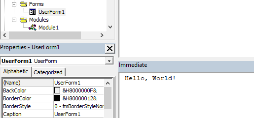
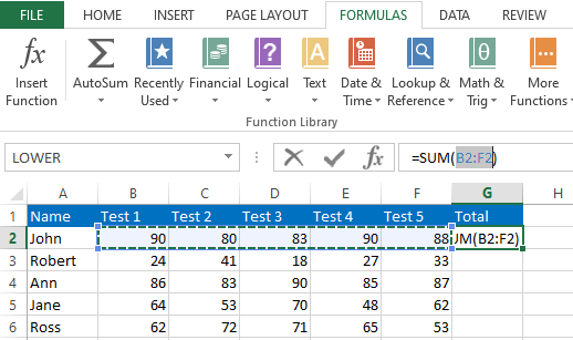
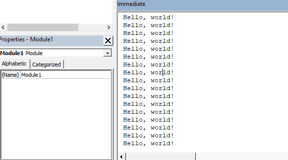
To test this macro, First I need to output something in the Immediate window. I will use the below macro to print “Hello, World!” hundred times in the immediate window.

Sub WriteHelloWorld()

     Dim i As Integer

     For i = 1 To 100
         Debug.Print "Hello, World!"
     Next i

End Sub

This is how the Immediate window looks like when run the above macro.

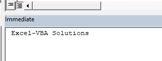
Now let's run the ClearImmediateWindow subroutine to see how it clears the immediate window.

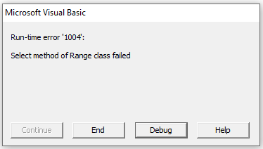
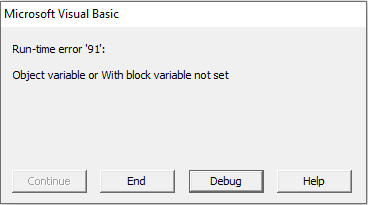
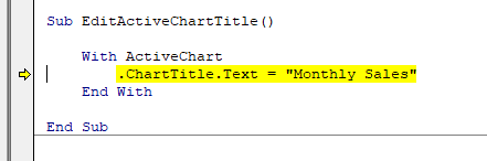
However, using the Application.Sendkeys method is not advisable. Because unexpected things can happen if a user interacts with the Excel application while running the program. For example a whole code in your modules can be deleted if accidentally selected a module instead of the immediate window. So this is not a robust code to use in a VBA application. I suggest not to use the Application.Sendkeys method if there are any other options.

How to Create a Column Chart Automatically Using VBA

Column charts are a chart type where data are represented from rectangles. In these charts, data are represented by vertical bars. Some people refer to these charts also as bar charts. But there is a difference between bar charts and column charts. If you interchange the x axis and y axis of a column chart then you will get a bar chart. Column charts make data easy to understand. Users will be able to understand the data at a glance when they are represented in column charts rather than in a written format. These charts are very helpful when we need to compare values of different categories. Column charts are more flexible than other chart types because you can plot lots of categories in one chart.

So in this lesson I’m going to show you how to insert a column chart using VBA. I will use this sample Excel sheet to show you how to do this. This worksheet lists sales data of each month of a company.

Assume the name of the worksheet is “Sales Data”. Then we can create a column chart automatically using the AddChart2 method available in VBA.

Sub CreateColumnChart()

     Dim WS As Worksheet

     Set WS = Worksheets("Sales Data")

     WS.Shapes.AddChart2(-1, xlColumn).Select
     ActiveChart.SetSourceData Source:=WS.Range("'Sales Data'!$A$1:$B$13")

End Sub

This is the result of the above subroutine.

In the above VBA code I have used single quotes for the worksheet name. It is because we have a space character in the worksheet name. But if you don’t have a space character in your worksheet name then you can write it without quotes. For example if your worksheet name is “Data” then you can rewrite that line as follows.

ActiveChart.SetSourceData Source:=WS.Range("Data!$A$1:$B$13")

Also you can revise the above code using the Worksheet.Name property as well. This is how you can do it.

Sub CreateColumnChart_Ex2()

     Dim WS As Worksheet

     Set WS = Worksheets("Sales Data")

     WS.Shapes.AddChart2(-1, xlColumn).Select
     ActiveChart.SetSourceData Source:=WS.Range("'" & WS.Name & "'" & "!$A$1:$B$13")

End Sub

I prefer this method because it is very easy to reuse or modify this code. For example if you want to use this for a different worksheet, then you need to change the worksheet name only in one line.

The AddChart2 method has several parameters. But all of them are optional. First parameter of the AddChart2 method is the style. In the above example, we used -1 as the first parameter of the AddChart2 method. If we set -1 as the style then we get the default style of the chart type specified in the second parameter. But we can create charts with various styles by changing this number. Here are some charts available in my Excel version.

Sub CreateColumnChart_Style209()

     Dim WS As Worksheet

     Set WS = Worksheets("Sales Data")

     WS.Shapes.AddChart2(209, xlColumn).Select
     ActiveChart.SetSourceData Source:=WS.Range("'" & WS.Name & "'" & "!$A$1:$B$13")

End Sub

Also Read
How to Add or Edit Chart Title Using VBA
Swap Axis of an Excel Chart Without Changing Excel Sheet Data
How to find the name of an active chart using VBA

Sub CreateColumnChart_Style208()

     Dim WS As Worksheet

     Set WS = Worksheets("Sales Data")

     WS.Shapes.AddChart2(208, xlColumn).Select
     ActiveChart.SetSourceData Source:=WS.Range("'" & WS.Name & "'" & "!$A$1:$B$13")

End Sub

Not all the styles available in every Excel version. So you should first find the style number of your preferred chart before developing the code. You can easily find the style number by using the record macro option available in Excel application. Start recording a macro and then create a column chart with a style you prefer. Then find the style number from the code generated. Check this post if you want to learn more about the record macro option available in the Excel application.

How to Record a Macro in Excel

Output Data in Excel VBA

VBA can display data in a few different ways.

• In the immediate window
• In a message box
• In an Excel sheet cell
• In a label/textbox control of a userform

Display data in the immediate window

This is a data output method commonly used by developers to test subroutines and functions while developing VBA applications. In this method you can write data into the immediate window using the Debug.Print method. Here is an example.

Sub PrintIntoImmediateWindow()

     Debug.Print "Hello, World!"

End Sub

This will write "Hello, World!" into the immediate window of the VBA editor.

Display data in a message box

From this method you can output data in a message box. We often use this option to display the program completion messages to the users.

Sub ShowDataInMessagebox()

     MsgBox "Completed!"

End Sub

Write data into a Excel sheet cell

You can also write data into Excel worksheets using VBA. This data output method is typically used when generating reports from VBA applications. You can generate sales reports, invoices etc through a VBA application using this method. Below is a very simplest example of this method. It will write "Hello, World!" into the cell A1 of the sheet1.

Sub PrintInWorksheet()

     Worksheets("Sheet1").Range("A1").Value = "Hello, World!"

End Sub

Output data in a label/textbox control of a userform

This data output method can be used when developing applications with one or more userforms. If you have a userform in your form, then you can display data inside label and textbox controls. Below is a sample form I created to show how to output data in a textbox control of a userform. I’m going to develop a simple code to print “Hello, World!” when a user clicks the “Print” button. Assume the name of the textbox is “txtMessage” and the name of the command button is “cmdPrint”.

Double click on the cmdPrint button. Then you will see this kind of click event in the userform code module.

Private Sub cmdPrint_Click()

End Sub

Then add the following code to that click event.

txtMessage.Value = "Hello, World!"

So the completed code should look like this.

Private Sub cmdPrint_Click()

     txtMessage.Value = "Hello, World!"

End Sub

Now when you click on the button, “Hello, World!” will be displayed in the textbox.

Also you can use TextBox.Text property instead of the value property as well.

txtMessage.Text = "Hello, World!"

Also read
Open and read text file using VBA
Convert an Excel Sheet to PDF Using VBA
Convert an Entire Workbook to a Single PDF File
Open files in a specific directory (folder)

How to Find the Style Number of an Excel Chart Using VBA

In this lesson you will learn how to find the style number of an Excel chart using VBA. Let’s consider this sample Excel sheet. This Excel sheet lists the number of sales for a few different items. Then an Excel chart has been used to visualize the sales of each item.

Now let’s see how we can find the style number of this Excel chart using VBA. I will show you how to find the style number of an active chart and of a chart by its name. In the first example you will be able to find the style number of a selected chart.

Find style number of an active chart using VBA

In this example we are going to find the style number of an active chart. To find the style number from this method, first click on the chart you want to find the style number of.

Then run this simple subroutine.

Sub FindChartStyleNo_Method1()

     MsgBox ActiveChart.ChartStyle

End Sub

This is the result obtained from the subroutine.

Find the style number of a chart by its name using VBA

From the previous subroutine we were able to get the style number of an active chart. You may know that each chart of a worksheet has a name. So in this next VBA macro we are going to find the style number of an Excel chart by its name. Remember that these names are not unique. Because users can create multiple charts with the same name.

Don’t know how to find the name of a chart? Check this post.
Find the name of a chart in Excel

Now let’s look at how to find the style number of a chart by its name. Assume that the name of our chart is “Chart 1”. Then we can find the style number of the chart using the following simple VBA macro.

Sub FindChartStyleNo_ByName()

     Dim MyChart As Chart

     Set MyChart = ActiveSheet.Shapes("Chart 1").Chart

     Debug.Print MyChart.ChartStyle

End Sub

If we run the above macro the style number of the Excel chart will be printed in the immediate window like this.

In this next example you will learn how to go through all the charts in the worksheet and print their names and style numbers. Here is the example sheet I’m going to use.

Let’s name this subroutine as FindChartStyleNo_AllCharts

Sub FindChartStyleNo_AllCharts()

End Sub

We need two variables for this subroutine.

Dim WS As Worksheet
Dim Sh As Shape

Next we can assign the worksheet to the WS variable as follows.

Set WS = Worksheets("Sales data")

Now we need to iterate through all the shapes of the worksheet. We can use For Each statement to do that.

For Each Sh In WS.Shapes

Next

Inside the For Each loop we need to separate only the charts. Because lots of other objects also belong to this shapes collection. So here we are going to use an If statement and the “Shape.Name” property to distinguish charts from other objects. Once charts are extracted then we can print the name and the style number in the immediate window.

If InStr(1, Sh.Name, "Chart", vbTextCompare) > 0 Then
     Debug.Print "Chart name - "; Sh.Name & " Style Number - " & Sh.Chart.ChartStyle
End If

So here is the full code of this subroutine.

Sub FindChartStyleNo_AllCharts()

     Dim WS As Worksheet
     Dim Sh As Shape

     Set WS = Worksheets("Sales data")

     For Each Sh In WS.Shapes
          If InStr(1, Sh.Name, "Chart", vbTextCompare) > 0 Then
               Debug.Print "Chart name - "; Sh.Name & " Style Number - " & Sh.Chart.ChartStyle
          End If
     Next

End Sub

This is the result of the above subroutine

But this method will only work when the user hasn't changed the chart name manually. If it is possible for the user to change the chart names then you can use the “Shapes.Type” property instead of the “Shapes.Name”. This is how you can modify the If statement section to use “Shapes.Type” property.

If Sh.Type = 3 Then
     Debug.Print "Chart type - "; Sh.Type & " Style Number - " & Sh.Chart.ChartStyle
End If

3 is the MsoShapeType value that represents the charts. Check below article from Microsoft documentation to see the values for different types of shapes.

MsoShapeType enumeration (Office)

Extract Numbers From a String Using VBA

When we develop VBA applications, sometimes we need to develop functions or subroutines to extract numbers from strings. So in this lesson you will learn a few different ways to extract numbers from a string using VBA.

Assume we have a string like this.

234sTsur45$p^

We are going to learn how to extract only 23445 from the above text string. There are few different ways to do this.

Method 1 - Using IsNumeric function

In this method we are going to use an inbuilt function called “IsNumeric” to extract only numbers from the string. Let’s name this subroutine as ExtractNumbers.

Sub ExtractNumbers()

End Sub

First we need to declare a few variables.

Dim MyString As String
Dim Tmp_Char As String
Dim ResultString As String
Dim i As Integer

Then we can assign our string to the MyString variable.

MyString = "234sTsur45$p^"

Next we need a For Next statement to iterate through each character of the string.

For i = 1 To Len(MyString)

Next i

Inside this For Next statement we can use the Mid function to extract each character one by one. Each character will be assigned to the Tmp_Char variable temporarily.

For i = 1 To Len(MyString)
     Tmp_Char = Mid(MyString, i, 1)
Next i

Now use IsNumeric function inside an If statement to check whether each character is a value or not. If the IsNumeric function returns true then we add that number to the ResultString variable.

For i = 1 To Len(MyString)
     Tmp_Char = Mid(MyString, i, 1)
     If IsNumeric(Tmp_Char) = True Then
         ResultString = ResultString & Tmp_Char
     End If
Next i

Want to learn more about the IsNumeric function? Check this post.

IsNumeric Function

This is the complete code of the first method.

Sub ExtractNumbers()

     Dim MyString As String
     Dim Tmp_Char As String
     Dim ResultString As String
     Dim i As Integer

     MyString = "234sTsur45$p^"

     For i = 1 To Len(MyString)
         Tmp_Char = Mid(MyString, i, 1)
         If IsNumeric(Tmp_Char) = True Then
             ResultString = ResultString & Tmp_Char
         End If
     Next i

     Debug.Print ResultString

End Sub

23445 will be printed in the immediate window when you run the above subroutine.

Method 2 - Using Select Case statement

In this method we are going to use Select Case statement instead of the If statement and IsNumeric function to extract numbers from the string. Below is the complete code of the second method.

Sub ExtractNumbers_Method2()

     Dim MyString As String
     Dim Tmp_Char As String
     Dim ResultString As String
     Dim i As Integer

     MyString = "234sTsur45$p^"

     For i = 1 To Len(MyString)
         Tmp_Char = Mid(MyString, i, 1)
         Select Case Tmp_Char
         Case 0 To 9
             ResultString = ResultString & Tmp_Char
         End Select
     Next i

     Debug.Print ResultString

End Sub

In this method Select Case statement is used to check whether the character is equal to value from 0 to 9. If the character is equal to value from 0 to 9 then those characters are appended to the ResultString.

Return a String From VBA function

Function is a block of code which can be used multiple times inside a program. So you can omit writing the same code again and again by using functions. Also programmers can break down the problem into smaller segments by using the functions. This will help programmers to organize their codes in a more meaningful way. Functions normally return a value to the sub or to the function called them. So in this lesson you will learn how to return a string from a VBA function. Here is the syntax of a function which returns a string.

Function FunctionName() as string

     '-----------------------
     'Codes of the function
     '-----------------------

     FunctionName = ResultString

End Function

Above is the syntax of a function which has no arguments. So let’s create a very simple function which outputs a string using the above syntax.

Function WebsiteName()

     WebsiteName = "Excel-VBA Solutions"

End Function

Above function returns the name of this website whenever it is called. Now you can call this function from a subroutine or from another function. This is how you can call the above function from a subroutine.

Sub Main()

     Dim Response As String

     Response = WebsiteName()

     Debug.Print Response

End Sub

When you run the subroutine, the name of the website will be printed in the immediate window.

Next let’s look at how to develop a function which has an argument. Here is the syntax of a function having one argument.

Function FunctionName (Argument as type) as string

     '-----------------------
     'Codes of the function
     '-----------------------

     FunctionName = ResultString

End Function

Type of the argument doesn’t need to be a string type. You can pass an argument of types such as Integer, Long, Boolean, Variant etc as well. Next let’s see how we can develop a function with an argument which returns a string. This is the sample Excel sheet I’m going to use for this example.

For this example I’m going to create a function which can return the employee name when we pass Id as the argument. Let’s name this new function as FindName. We need to use a For Next statement inside our function to get the expected result. Assume the name of the worksheet is Data. You can develop the function as below to get the name of the employee when passing the Id as argument.

Function FindName(Id_no As Long) As String

     Dim WS As Worksheet
     Dim i As Integer
     Dim LastRow As Integer

     Set WS = Worksheets("Data")
     LastRow = WS.Cells.Find("*", [A1], , , xlByRows, xlPrevious).Row

     For i = 2 To LastRow
         If WS.Range("A" & i).Value = Id_no Then
             FindName = WS.Range("B" & i).Value
             Exit Function
         End If
     Next i

     'If id not found
     FindName = ""

End Function

So above is an example VBA function with an argument which returns a string. Program check for the matching id while iterating through each row number. If it finds a matching id then the function will return the corresponding name. Exit function statement is used to stop executing other lines of code once a function finds a match. If the Id is not found, the function will be executed til the end and will return an empty string. Here is how you can use the above function inside a subroutine.

Sub EmployeeData()

     Dim EmployeeName As String
     Dim IdNumber As Long

     IdNumber = 135421
     EmployeeName = FindName(IdNumber)

     MsgBox EmployeeName

End Sub

Name of the relevant employee will be displayed in a message box when the code is executed.

This is what happens when you pass an Id which is not available in the worksheet.

Sub EmployeeData()

     Dim EmployeeName As String
     Dim IdNumber As Long

     IdNumber = 135429
     EmployeeName = FindName(IdNumber)

     MsgBox EmployeeName

End Sub

How to Sum a Row in Excel

In this lesson you will learn how to sum a row in Excel. I will show you two methods to get the total of an Excel row. Let’s consider this sample Excel sheet. We have names of students in column A. Then we have marks of five tests in the next five columns. Assume we want to calculate the total of five tests for each student.

Method 1

In the above example Excel sheet we want to get the sum of each row to the column G. First let’s look at how to sum a row in Excel for one row. Then we can apply similar formulas for other rows as well. Here are the steps to follow. First click on the G2 cell. Next go to the “FORMULAS” tab in the Excel ribbon.

Then click on the AutoSum

Then you will see that the Sum formula is automatically inserted to the selected cell.

Now press enter. Total value will be calculated like this. So this is one way to sum a row in Excel.

Next let’s see how we can apply similar formulas to other rows easily. To do that, first take the mouse pointer to the right bottom corner of the G2 cell. Mouse pointer will change to a + mark. Then drag the mouse upto 10th row while holding down the left mouse button. Then the total for each row will be calculated like this.

You can use this same technique to sum a column as well. Only difference is you need to select a cell bottom to the data set. For an example you can select cell B11.

Method 2

Next let’s look at the second method to sum a row in Excel. I will use this sample Excel sheet to explain this second method.

Suppose we want to get the sum of the 3rd row. If we use this second method we can get the result to any row except row 3. Because if we try to get the result value in the same row then we will get a Circular references error.

To avoid this error let’s get the result in the cell A5. To get the result using the second method enter the following formula in cell A5. Note that you can enter this formula in any cell which is not on row 3.

=SUM(3:3)

Here is the result of the above formula.

You can use this method to get the sum of the entire row. Total will be calculated even if you have some text in between.

How to Highlight Duplicate Values in Excel

In this post you will learn about how to highlight duplicate values in Excel. Let’s consider this sample data.

This Excel sheet contains a list of codes in column A. Assume we want to know whether there are duplicated codes in the list and highlight them. Instead of manually examining, we can use conditional formatting available in the Excel application to highlight the duplicates. Follow the below steps.

First select the data set.

Then select the “Home” tab from the Excel ribbon.

Click on the “Conditional Formatting” in the style group.

Now take the cursor on top of the “Highlight Cells Rules” menu. Then a submenu will appear to the right. Click on the “Duplicate Values” from that submenu.

Then the Duplicate values window will open like this. Select “Duplicate” from the first dropdown. I will select “Light Red Fill with Dark Red Text” from the second dropdown. You can select any other format or custom format from the list.

Then click the "OK" button. Duplicate codes will be highlighted like this.

In the above example we selected a range to apply the conditional formatting. However if you need you can add the conditional formatting to the entire column as well. To do that you need to change only one step. When selecting the data, select the entire column instead of the range. Below image shows how you should select the column.

Select All Cells Using VBA

In this post you will learn about different ways to select all cells of a worksheet using VBA. When developing VBA macros you may need the VBA program to select all cells of a worksheet. For an example you might need to select all cells before printing the Excel sheet. There are many ways to select all cells of an Excel worksheet using VBA. In this lesson you will learn four different ways to select all cells of an Excel sheet.

Table of contents
Select all cells using Cells.Select Method
Select all cells using UsedRange property
Select all cells using last row and column numbers
Select all cells using CurrentRegion property

Cells.Select Method

This is the simplest way to select all the cells of an Excel worksheet using VBA. If you want to select all the cells of the activesheet then you can use the below code to do that.

Sub SelectAllCells_Method1_A()

     ActiveSheet.Cells.Select

End Sub

However keep in mind that this method will select all cells of the worksheet including the empty cells.

Sometimes you may need to select all cells of a specific sheet of a workbook which contains multiple worksheets. Then you can refer to that specific sheet by its name. If the name of the sheet is “Data” then you can modify the above VBA macro as follows.

Sub SelectAllCells_Method1_B()

     Dim WS As Worksheet

     Set WS = Worksheets("Data")

     WS.Activate
     WS.Cells.Select

End Sub

Note that it is important to use the Worksheet.Activate method before selecting all cells. Because the VBA program can’t select cells of a worksheet which is not active. Program will throw an error if you try to select cells of a worksheet which is not active.

UsedRange Method

Above macros select all the cells of the worksheet. So VBA programs select cells even beyond the last row and column having data. But what if you want to select all the cells only inside the range you have used? For that you can use Worksheet.UsedRange property.

Sub SelectAllCells_Method2()

     Dim WS As Worksheet

     Set WS = Worksheets("Data")

     WS.Activate
     WS.UsedRange.Select

End Sub

Above VBA code will select all the cells inside the range you have used.

Select all cells using last row and column numbers

Also there is an alternative way to do this using VBA. First we can find the row number of the bottom most cell having data. Next we can find the column number of the rightmost cell having data. Then we can select the complete range from cell A1 to cell with those last row and column numbers using VBA. Here is how we can do it.

Sub SelectAllCells_Method3()

     Dim WS As Worksheet
     Dim WS_LastRow As Long
     Dim WS_LastColumn As Long
     Dim MyRange As Range

     Set WS = Worksheets("Data")

     WS_LastRow = WS.Cells.Find("*", [A1], , , xlByRows, xlPrevious).Row
     WS_LastColumn = WS.Cells.Find("*", [A1], , , xlByColumns, xlPrevious).Column

     Set MyRange = WS.Range(Cells(1, 1), Cells(WS_LastRow, WS_LastColumn))

     WS.Activate
     MyRange.Select

End Sub

There is one difference between those last two methods. If you use the last row and column numbers method, the range will be selected from cell A1. But if you use the UsedRange property then the range will be started from the first cell with the data. However you can also modify the last row and column numbers macro to get the same result as the Worksheet.UsedRange property method. But it will be a little more complicated.

Using CurrentRegion Property

We can also use the Range.CurrentRegion property to select all cells of an Excel worksheet. We can easily do that by making a slight change to the UsedRange method. Here is how we can select all cells using the CurrentRegion property.

Sub SelectAllCells_Method4()

     Dim WS As Worksheet

     Set WS = Worksheets("Data")

     WS.Activate
     WS.Range("A1").CurrentRegion.Select

End Sub

However there is one limitation in this method. If you have empty rows in your worksheet, then the VBA program will select cells only upto that row.

How to Add or Edit Chart Title Using VBA

Typically, If you have titles in your data, Excel will automatically add a relevant title to the chart. But if no titles present in the data or if titles are not selected when inserting the chart, then the created chart will not have a title. And sometimes you might need to add a different title to the chart than present in the data. So in this lesson you will learn how to add or edit a chart title using VBA. Let’s consider this sample chart.

This chart was created from the data below.

If you look at the above Excel line chart, you will notice that the chart was created with the default title text called “Chart Title”. So in this lesson first let’s look at how to edit an existing title like that.

Assume you want to edit a title of an active chart. You can do it very easily as shown below.

Sub EditActiveChartTitle()

     With ActiveChart
         .ChartTitle.Text = "Monthly Sales"
     End With

End Sub

However, for this macro to be worked, your chart should be in an active state(Selected). Otherwise the VBA program will throw an error like this.

But if you know the name of the chart then you can develop a VBA code to edit the title of the chart independent of whether it is active or not. For example, the subroutine below will change the chart title to “Monthly Sales” of a chart called “Chart 2”.

Sub EditTitleFromChartName()

     Dim MyChart As Chart

     Set MyChart = ActiveSheet.Shapes("Chart 2").Chart
     With MyChart
         .ChartTitle.Text = "Monthly Sales"
     End With

End Sub

Don’t know how to find the name of a chart? Check this post to learn how.
Find the name of a chart in Excel

Sometimes you might need to add a chart title to a chart which doesn’t have any title. Here is an example. This chart doesn’t have any title. As mentioned above this can happen if no titles present in the data or if the user doesn’t select the titles when inserting the chart. So let’s see how we can add a title to it.

To add a chart title, we need to do a very simple change to the above VBA code we used to edit the title. The only change needed is we should make the HasTitle property from False to True. So this is how you can add a chart title to an active chart by changing the HasTitle property.

Sub AddChartTitle()

     With ActiveChart
         .HasTitle = True
         .ChartTitle.Text = "Monthly Sales"
     End With

End Sub

Also If you know the name of the chart you want to add the title then you can change the above VBA code like this.

Sub AddTitleFromChartName()

     Dim MyChart As Chart

     Set MyChart = ActiveSheet.Shapes("Chart 2").Chart
     With MyChart
         .HasTitle = True
         .ChartTitle.Text = "Monthly Sales"
     End With

End Sub

Here is the result of the above macros.

Also Read
How to create a line chart automatically - Excel VBA
Swap Axis of an Excel Chart Without Changing Excel Sheet Data
Formatting Excel Line Charts Using VBA