Want to become an expert in VBA? So this is the right place for you. This blog mainly focus on teaching how to apply Visual Basic for Microsoft Excel. So improve the functionality of your excel workbooks with the aid of this blog. Also ask any questions you have regarding MS Excel and applying VBA. We are happy to assist you.

How to Add or Edit Chart Title Using VBA

Typically, If you have titles in your data, Excel will automatically add a relevant title to the chart. But if no titles present in the data or if titles are not selected when inserting the chart, then the created chart will not have a title. And sometimes you might need to add a different title to the chart than present in the data. So in this lesson you will learn how to add or edit a chart title using VBA. Let’s consider this sample chart.

Sample chart

This chart was created from the data below.

Sample data

If you look at the above Excel line chart, you will notice that the chart was created with the default title text called “Chart Title”. So in this lesson first let’s look at how to edit an existing title like that.

Assume you want to edit a title of an active chart. You can do it very easily as shown below.

Sub EditActiveChartTitle()

     With ActiveChart
         .ChartTitle.Text = "Monthly Sales"
     End With

End Sub

However, for this macro to be worked, your chart should be in an active state(Selected). Otherwise the VBA program will throw an error like this.

Program will throw an error if the chart is not selected
Error line

But if you know the name of the chart then you can develop a VBA code to edit the title of the chart independent of whether it is active or not. For example, the subroutine below will change the chart title to “Monthly Sales” of a chart called “Chart 2”.

Sub EditTitleFromChartName()

     Dim MyChart As Chart

     Set MyChart = ActiveSheet.Shapes("Chart 2").Chart
     With MyChart
         .ChartTitle.Text = "Monthly Sales"
     End With

End Sub

Don’t know how to find the name of a chart? Check this post to learn how.
Find the name of a chart in Excel

Sometimes you might need to add a chart title to a chart which doesn’t have any title. Here is an example. This chart doesn’t have any title. As mentioned above this can happen if no titles present in the data or if the user doesn’t select the titles when inserting the chart. So let’s see how we can add a title to it.

Chart without a title

To add a chart title, we need to do a very simple change to the above VBA code we used to edit the title. The only change needed is we should make the HasTitle property from False to True. So this is how you can add a chart title to an active chart by changing the HasTitle property.

Sub AddChartTitle()

     With ActiveChart
         .HasTitle = True
         .ChartTitle.Text = "Monthly Sales"
     End With

End Sub

Also If you know the name of the chart you want to add the title then you can change the above VBA code like this.

Sub AddTitleFromChartName()

     Dim MyChart As Chart

     Set MyChart = ActiveSheet.Shapes("Chart 2").Chart
     With MyChart
         .HasTitle = True
         .ChartTitle.Text = "Monthly Sales"
     End With

End Sub

Here is the result of the above macros.

VBA Macro will add the title to the chart

Also Read
How to create a line chart automatically - Excel VBA
Swap Axis of an Excel Chart Without Changing Excel Sheet Data
Formatting Excel Line Charts Using VBA

How to Insert a Pie Chart Using VBA

In this lesson you will learn how to insert a pie chart automatically using VBA. Pie charts are very useful in data visualization. Because from a pie chart, users can get a clear picture about the data at a glance. So let's use the below sample data to see how to create a pie chart automatically using VBA. This table shows the profits of different branches of a company.

sample data sheet

Assume name of the worksheet is "Sheet1". As we have data in the range A1:B6, we can insert the pie chart automatically using VBA as follows.

Sub Create3DPieChart()

     Dim WS As Worksheet

     Set WS = Worksheets("Sheet1")

     WS.Shapes.AddChart2(-1, xl3DPie).Select
     ActiveChart.SetSourceData Source:=Range(WS.Name & "!$A$1:$B$6")

End Sub

Here is the result of the above macro.

VBA Program will insert the default pie chart

This is the syntax of the AddChart2 method.

Syntax of the AddChart2 method

Note that all the parameters are optional for the AddChart2 method. In the above VBA code we have set “-1” as the style and the “xl3DPie” as the xlChartType. Since we have used “-1” Excel will create the default style of the xl3DPie chart type.

Check this post if you want to learn more about the AddChart2 method.

AddChart2 Method

Next let’s see how we can insert a 2D Pie chart by modifying the above VBA code. To do that we need to only change the second parameter of the AddChart2 method.

Sub Create2DPieChart()

     Dim WS As Worksheet

     Set WS = Worksheets("Sheet1")

     WS.Shapes.AddChart2(-1, xlPie).Select
     ActiveChart.SetSourceData Source:=Range(WS.Name & "!$A$1:$B$6")

End Sub

If you run the above macro, a 2D Pie chart will be created like this.

2D Pie chart inserted by the VBA macro

Sometimes you may want to insert a pie chart with a different style. For an example, suppose you want to create a pie chart with a dark background. This is how you can do it in Excel 2013.

Sub Create3DPieChart_DarkBackground()

     Dim WS As Worksheet

     Set WS = Worksheets("Sheet1")

     WS.Shapes.AddChart2(262, xl3DPie).Select
     ActiveChart.SetSourceData Source:=Range(WS.Name & "!$A$1:$B$6")

End Sub
Pie chart with dark background

Note that we only changed the style number to create this new chart.

However not all the chart styles are available for every Excel version. Because newer Excel versions have more features than previous versions. So how do we find the exact style number of our prefered chart? You can find that by using the Record Macro function.

Follow these simple steps to find the style number of your preferred chart.

Go to the developer tab and click on Record Macro.

Go to developer tab and click record macro

Give the macro a suitable name and click OK. Also you can decide where you want to store the VBA macro by selecting an option from the “Store macro in” dropdown.

Give the macro a name and click OK

Then select the data.

Select data

Go to the Insert tab and select the chart you want to create.

Select the chart you want to insert

Now select a chart design from the list. I will select the 3rd design from the top row for this example.

Select a chart design from the list

Next, go to the “Developer” tab again and click “Stop Recording”.

Stop recording

Click on the “Visual Basic” to view the code.

Click on the visual basic to view the VBA code

Now you can incorporate these circled values to your code to create a chart automatically with similar style.

Generated VBA code

Check this post if you want to learn more about recording a macro in Excel.

Record a Macro in Excel

VBA - Get Unique Values From Column Into Array

When developing Excel VBA programs, sometimes we need to get unique values from a column into an array. Particularly when creating dynamic lists for dropdowns or generating reports. For an example assume you have a dropdown in your VBA program. Suppose that it needs to be updated with the data entered by the user. If the related data is stored in a column, then we can use that column to populate the dropdown. But what, if values are repeated in the column? We don’t show duplicate values in a dropdown list. So then you need to get only unique values to the dropdown. To do that first we can add unique values from column to an array. Then we can easily create the list of the dropdown using that array. So in this lesson you will learn how to populate an array from unique values of a given column. Also I’m going to develop a VBA function for this. So you can readily use it in your VBA programs.

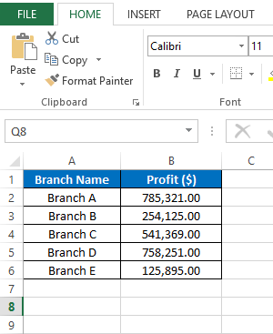
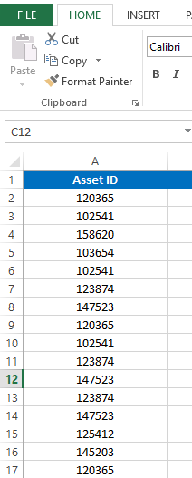
Below is the list I’m going to use for this lesson. It is a list of asset ids. And they are listed in column A.

List of asset ids

This is not a list of unique values. Because some asset ids are repeated in the column. So now let’s see how we can add only unique values from this column to a VBA array. I’m going to create a custom VBA function for this.

Function GetUniqueValuesFromColumnIntoArray(WS As Worksheet, ColumnName As String) As String()

End Function

This VBA function has two parameters. WS and ColumnName. I added these two parameters to input the worksheet name and the column. So you can reuse this for your worksheets easily. Also note that the return type of the VBA function is String(). This is because the function needs to return an array. Want to learn more about returning an array from a VBA function? Check this post.

How to Return an Array From VBA Function

Now we have declared the function name with parameters. Next we need to declare a few variables.

Dim WS_ColumnName_LastRow As Long
Dim i As Long
Dim j As Long
Dim Counter As Long
Dim AllValues() As String
Dim UniqueValues() As String
Dim ValueFound As Boolean

AllValues() array will hold all the values from the column. The UniqueValues() variable will hold only the unique values from the column.

Next, find the last row of the list.

With WS
     WS_ColumnName_LastRow = .Cells(.Rows.Count, ColumnName).End(xlUp).Row
End With

Size the “AllValues” dynamic array that has already been formally declared.

ReDim AllValues(1 To WS_ColumnName_LastRow)

Populate the AllValues array using a For Next statement.

For i = 1 To WS_ColumnName_LastRow
     AllValues(i) = WS.Range(ColumnName & i).Value
Next i

Then we need to size the UniqueValues array. Here we size the UniqueValues array to the same size of the AllValues array. Because at this moment we don’t know how many unique values we will have in the array. Once all the unique values are populated then we can resize the array to appropriate size.

ReDim UniqueValues(1 To WS_ColumnName_LastRow)

Add the first element from AllValues to the UniqueValues array.

UniqueValues(1) = AllValues(1)

Next we use a nested For Next statement to find unique values.

Counter = 1
For i = 1 To WS_ColumnName_LastRow
     ValueFound = False
     For j = 1 To Counter
          If StrComp(AllValues(i), UniqueValues(j), vbTextCompare) = 0 Then
              ValueFound = True
              Exit For
          End If
     Next j
     If ValueFound = False Then
          Counter = Counter + 1
          UniqueValues(Counter) = AllValues(i)
     End If
Next i

In the above code, the outer For Next statement is used to iterate through the elements of the AllValues array.

For i = 1 To WS_ColumnName_LastRow

Next i

Then this inner For Next statement is used to iterate through existing(Newly adding) elements of the UniqueValues array.

For j = 1 To Counter

Next j

StrComp function returns 0 if the elements of the two arrays are matching.

StrComp(AllValues(i), UniqueValues(j), vbTextCompare)

Here the variable ValueFound is used as a flag.

If the value is not found among the elements of the UniqueValues array, then this new value is added as the next element.

If ValueFound = False Then
     Counter = Counter + 1
     UniqueValues(Counter) = AllValues(i)
End If

Once all the unique values are collected to the UniqueValues array, we can resize the UniqueValues array as follows. Use the Preserve keyword to keep the existing values while resizing the array. If not, all the values will be erased.

ReDim Preserve UniqueValues(1 To Counter)

Finally, the function returns the UniqueValues array as the output.

GetUniqueValuesFromColumnIntoArray = UniqueValues

And Below is the full code of the function.

Function GetUniqueValuesFromColumnIntoArray(WS As Worksheet, ColumnName As String) As String()

     Dim WS_ColumnName_LastRow As Long
     Dim i As Long
     Dim j As Long
     Dim Counter As Long
     Dim AllValues() As String
     Dim UniqueValues() As String
     Dim ValueFound As Boolean

     With WS
          WS_ColumnName_LastRow = .Cells(.Rows.Count, ColumnName).End(xlUp).Row
     End With

     ReDim AllValues(1 To WS_ColumnName_LastRow)

     For i = 1 To WS_ColumnName_LastRow
          AllValues(i) = WS.Range(ColumnName & i).Value
     Next i

     ReDim UniqueValues(1 To WS_ColumnName_LastRow)
     UniqueValues(1) = AllValues(1)
     Counter = 1
     For i = 1 To WS_ColumnName_LastRow
          ValueFound = False
          For j = 1 To Counter
               If StrComp(AllValues(i), UniqueValues(j), vbTextCompare) = 0 Then
                    ValueFound = True
                    Exit For
               End If
          Next j
          If ValueFound = False Then
               Counter = Counter + 1
               UniqueValues(Counter) = AllValues(i)
          End If
     Next i

     ReDim Preserve UniqueValues(1 To Counter)
     GetUniqueValuesFromColumnIntoArray = UniqueValues

End Function

You can use this function inside a subroutine like this. Assume the name of the worksheet is “Data”.
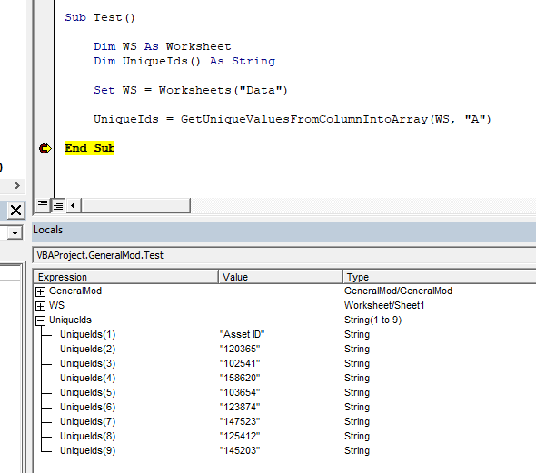
Sub Test()

     Dim WS As Worksheet
     Dim UniqueIds() As String

     Set WS = Worksheets("Data")

     UniqueIds = GetUniqueValuesFromColumnIntoArray(WS, "A")

End Sub

Add a breakpoint at “End Sub” and run the program. Then view the UniqueIds array in the “Locals” window.

View the array with unique values

The example worksheet we considered above has a header in row 1. Therefore we have the header “Asset ID” also in the result array. But sometimes you might need to populate unique values into an array without the header. There are few different ways to achieve this. Also you can do it by changing the function or changing the subroutine. In here I will show you how to modify the subroutine to get unique values without the header.

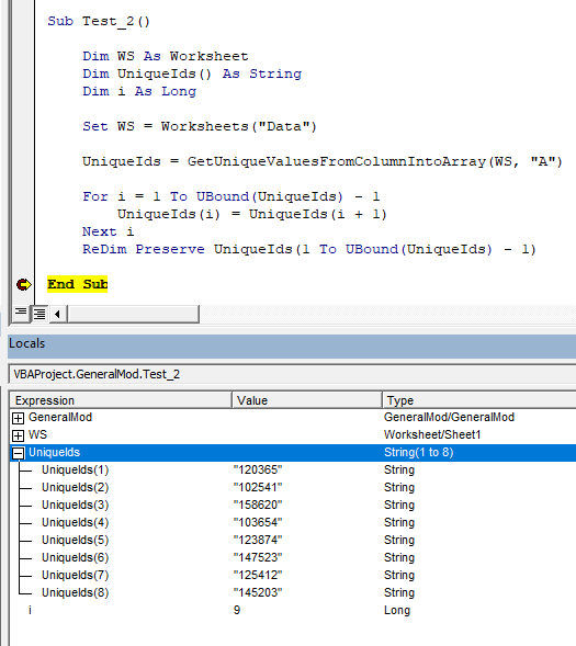
Here is how we can modify the subroutine. Once we get the unique values to the array, we can iterate through all the elements using a For Next statement. While loop through the elements we can decrement the index of each and every element by 1. Then the first element which is the header will be removed. Finally we can resize the array to one less than the original size. To keep the current values use the Preserve keyword when resizing.

Sub Test_2()

     Dim WS As Worksheet
     Dim UniqueIds() As String
     Dim i As Long

     Set WS = Worksheets("Data")

     UniqueIds = GetUniqueValuesFromColumnIntoArray(WS, "A")

     For i = 1 To UBound(UniqueIds) - 1
          UniqueIds(i) = UniqueIds(i + 1)
     Next i

     ReDim Preserve UniqueIds(1 To UBound(UniqueIds) - 1)

End Sub

Below is the outcome of the above subroutine.

Adding unique values from a column into an array

Also Read
Fill a Listbox From an Array
Transposing an Array in VBA
Re-size Dynamic Arrays
Quickly Write Multidimensional Array to Excel Range

Contact Form

Name

Email *

Message *