In this lesson you will learn how to insert a pie chart automatically using VBA. Pie charts are very useful in data visualization. Because from a pie chart, users can get a clear picture about the data at a glance. So let's use the below sample data to see how to create a pie chart automatically using VBA. This table shows the profits of different branches of a company.
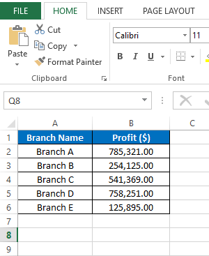
Assume name of the worksheet is "Sheet1". As we have data in the range A1:B6, we can insert the pie chart automatically using VBA as follows.
Dim WS As Worksheet
Set WS = Worksheets("Sheet1")
WS.Shapes.AddChart2(-1, xl3DPie).Select
ActiveChart.SetSourceData Source:=Range(WS.Name & "!$A$1:$B$6")
End Sub
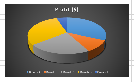
Here is the result of the above macro.

This is the syntax of the AddChart2 method.
Note that all the parameters are optional for the AddChart2 method. In the above VBA code we have set “-1” as the style and the “xl3DPie” as the xlChartType. Since we have used “-1” Excel will create the default style of the xl3DPie chart type.
Check this post if you want to learn more about the AddChart2 method.
Next let’s see how we can insert a 2D Pie chart by modifying the above VBA code. To do that we need to only change the second parameter of the AddChart2 method.
Dim WS As Worksheet
Set WS = Worksheets("Sheet1")
WS.Shapes.AddChart2(-1, xlPie).Select
ActiveChart.SetSourceData Source:=Range(WS.Name & "!$A$1:$B$6")
End Sub
If you run the above macro, a 2D Pie chart will be created like this.

Sometimes you may want to insert a pie chart with a different style. For an example, suppose you want to create a pie chart with a dark background. This is how you can do it in Excel 2013.
Dim WS As Worksheet
Set WS = Worksheets("Sheet1")
WS.Shapes.AddChart2(262, xl3DPie).Select
ActiveChart.SetSourceData Source:=Range(WS.Name & "!$A$1:$B$6")
End Sub
Note that we only changed the style number to create this new chart.
However not all the chart styles are available for every Excel version. Because newer Excel versions have more features than previous versions. So how do we find the exact style number of our prefered chart? You can find that by using the Record Macro function.
Follow these simple steps to find the style number of your preferred chart.
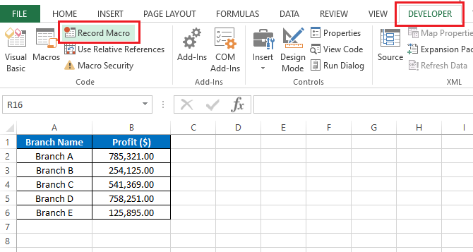
Go to the developer tab and click on Record Macro.
Give the macro a suitable name and click OK. Also you can decide where you want to store the VBA macro by selecting an option from the “Store macro in” dropdown.

Then select the data.

Go to the Insert tab and select the chart you want to create.

Now select a chart design from the list. I will select the 3rd design from the top row for this example.

Next, go to the “Developer” tab again and click “Stop Recording”.

Click on the “Visual Basic” to view the code.
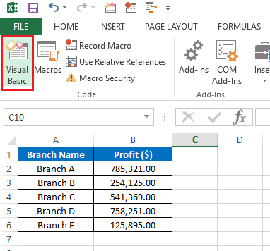
Now you can incorporate these circled values to your code to create a chart automatically with similar style.

Check this post if you want to learn more about recording a macro in Excel.