Column charts are a chart type where data are represented from rectangles. In these charts, data are represented by vertical bars. Some people refer to these charts also as bar charts. But there is a difference between bar charts and column charts. If you interchange the x axis and y axis of a column chart then you will get a bar chart. Column charts make data easy to understand. Users will be able to understand the data at a glance when they are represented in column charts rather than in a written format. These charts are very helpful when we need to compare values of different categories. Column charts are more flexible than other chart types because you can plot lots of categories in one chart.
So in this lesson I’m going to show you how to insert a column chart using VBA. I will use this sample Excel sheet to show you how to do this. This worksheet lists sales data of each month of a company.

Assume the name of the worksheet is “Sales Data”. Then we can create a column chart automatically using the AddChart2 method available in VBA.
Dim WS As Worksheet
Set WS = Worksheets("Sales Data")
WS.Shapes.AddChart2(-1, xlColumn).Select
ActiveChart.SetSourceData Source:=WS.Range("'Sales Data'!$A$1:$B$13")
End Sub
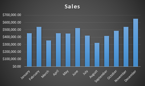
This is the result of the above subroutine.

In the above VBA code I have used single quotes for the worksheet name. It is because we have a space character in the worksheet name. But if you don’t have a space character in your worksheet name then you can write it without quotes. For example if your worksheet name is “Data” then you can rewrite that line as follows.
Also you can revise the above code using the Worksheet.Name property as well. This is how you can do it.
Dim WS As Worksheet
Set WS = Worksheets("Sales Data")
WS.Shapes.AddChart2(-1, xlColumn).Select
ActiveChart.SetSourceData Source:=WS.Range("'" & WS.Name & "'" & "!$A$1:$B$13")
End Sub
I prefer this method because it is very easy to reuse or modify this code. For example if you want to use this for a different worksheet, then you need to change the worksheet name only in one line.
The AddChart2 method has several parameters. But all of them are optional. First parameter of the AddChart2 method is the style. In the above example, we used -1 as the first parameter of the AddChart2 method. If we set -1 as the style then we get the default style of the chart type specified in the second parameter. But we can create charts with various styles by changing this number. Here are some charts available in my Excel version.
Dim WS As Worksheet
Set WS = Worksheets("Sales Data")
WS.Shapes.AddChart2(209, xlColumn).Select
ActiveChart.SetSourceData Source:=WS.Range("'" & WS.Name & "'" & "!$A$1:$B$13")
End Sub
Also Read
How to Add or Edit Chart Title Using VBA
Swap Axis of an Excel Chart Without Changing Excel Sheet Data
How to find the name of an active chart using VBA
Dim WS As Worksheet
Set WS = Worksheets("Sales Data")
WS.Shapes.AddChart2(208, xlColumn).Select
ActiveChart.SetSourceData Source:=WS.Range("'" & WS.Name & "'" & "!$A$1:$B$13")
End Sub

Not all the styles available in every Excel version. So you should first find the style number of your preferred chart before developing the code. You can easily find the style number by using the record macro option available in Excel application. Start recording a macro and then create a column chart with a style you prefer. Then find the style number from the code generated. Check this post if you want to learn more about the record macro option available in the Excel application.