How to Insert Modules in Excel VBA Projects

VBA (Visual Basic for Applications) is a powerful tool in Excel that allows users to automate tasks and enhance functionality. In this guide, we will walk you through the process of inserting a module into your Excel VBA project.

Step 1: Accessing the Developer Tab

Go to the "Developer" tab on the Excel ribbon. If you don't see the Developer tab, you may need to enable it in Excel's options. Check this previous post to learn how to enable the Developer tab in your Excel application.

How to show the Developer tab in Excel

Step 2: Opening the VBA Editor

Click on "Visual Basic" in the Developer tab. This action opens the VBA Editor, where you can create and manage your VBA code.

Step 3: Selecting the Workbook

In the Project Explorer window on the left, click on the workbook for which you want to insert a module. This step is crucial if you have multiple workbooks open.

In this example I’m going to insert the module to the VBA project of the Book2 file.

Step 4: Inserting a Module

From the menu, select "Insert" and then choose "Module." This command adds a new module under the selected workbook in the Project Explorer.

Step 5: Opening the Module

When you insert a new module, that module will be automatically open in the central editing area. If you have multiple modules in one or more VBA projects and if you want to add/edit or view code in a particular module, then double-click on the module you want. This action opens that particular module in the central editing area, allowing you to add/edit or view your VBA code.

Inserting a module provides a foundation for incorporating custom automation and functionalities into your Excel projects. With this guide, you can now easily insert VBA modules into your workbooks.

Populate Userform Listbox from Range

In this lesson you will learn how to populate a userform listbox with a range. In VBA (Visual Basic for Applications), a list box is a graphical user interface control that allows users to make a selection from a list of items. It is commonly used in user forms to display data or present a list of options from which the user can choose. When it is used to present a list from which the user can select, the selected item or items in the list box can then be used for further processing in the other VBA codes associated with controls such as command buttons. Or by codes even associated with events such as listbox_click events etc.

A list box can contain a collection of items, typically displayed in a vertical list. These items can be static (defined at design time) or dynamic (populated at runtime). In this example we will use a collection of static items stored in a worksheet. If you want to populate the list box with a dynamic data set, then the best option is to populate data from an array. This post explains how to populate a listbox from an array.

Fill a Listbox From an Array

Name of this worksheet is “EmployeeData”. This worksheet contains Full Name, Job Title, Department, Employee ID and Date of Joining for 10 employees. Now let’s see how we can populate these data into a userform listbox. This is the listbox we are going to use for this example. Name of the form is frmEmployeeData and name of the listbox is lstEmployeeData.

Now we can write the vba code inside the UserForm_Initialize event to populate the listbox with Excel range.

Private Sub UserForm_Initialize()

End Sub

This is how we can populate the list with the above Excel range.

Private Sub UserForm_Initialize()

     With lstEmployeeData
         .ColumnCount = 5
         .RowSource = "=EmployeeData!A1:E11"
     End With

End Sub

This is how the listbox is populated from the Excel data range.

Remember that you can’t use worksheet names having spaces.In the above example we use an Excel sheet called “EmployeeData”. Assume our worksheet name is “Employee Data”. Then we can’t modify the code as follows.

Private Sub UserForm_Initialize()

     With lstEmployeeData
         .ColumnCount = 5
         .RowSource = "=Employee Data!A1:E11"
     End With

End Sub

Because then it will throw an error like this.

How to Test a Custom VBA Function in Immediate Window

In this post I will show you how you can test a custom function in the immediate window. When you develop advanced VBA applications with multiple subroutines and functions you may need to test them while developing the code. Then you can use this technique to test individual functions without running the whole program. So now let’s look at how to call a user defined function from the immediate window. Here is a simple custom function I created to use as an example.

Function SumValues()

     Dim a As Long
     Dim b As Long
     Dim c As Long
     Dim Result As Long

     a = 1000
     b = 2000
     c = 3500

     Result = a + b + c
     SumValues = Result

End Function

This is a very simple function which returns the sum of three values. Now let’s see how we can test this function in the immediate window. First open the immediate window if it is not already opened.

How to Show Immediate Window in VBA Environment

When you open the immediate window you can test the custom function using one of the below two methods.

Method 1

Enter the function name followed by a question mark.

?SumValues

So here is the result you will get.

That's one way to call a custom function from the immediate window.

Method 2

In this method we are going to use the debug.print method to print the result of the function in the immediate window.

This is how you can test a custom VBA function in the immediate window using this second method.

debug.Print SumValues()

Also read
How to Return an Array From VBA Function
How to Pass an Array to a VBA Function
How to Search For Multiple Strings Using VBA InStr Function
BESSELJ Function

How to Clear the Immediate Window Using VBA

A VBA program can have multiple subroutines and functions. If you are a programmer you will need to test these subroutines and functions while developing the VBA code. Then the immediate window is a helpful tool you can use to test your components. If it is a subroutine, then you can print your variables using debug.print method to ensure whether they are calculated correctly. If it is a function you can print the return value in the immediate window.

From one of our previous posts we learnt how to output data in VBA using a few different ways. In that post you can find how to output data to Immediate window using VBA.

Output data in Excel VBA

So today I'm going to show you how to clear the immediate window automatically using VBA. You may know how to clear it manually. If you don't know, follow these simple steps. First select everything in the immediate window. Then press the delete key on the keyboard to delete everything. If the immediate window is not visible you can use shortcut keys “Ctrl + G” to view the immediate window. Also if the cursor is in a different window than the immediate window, and if you press the above shortcut keys, then the cursor will move to the immediate window giving you access to the immediate window.

Now let’s look at how we can clear the immediate window using VBA. We can use the Application.Sendkeys method to clear the immediate window using VBA. Application.Sendkeys method lets us send keystrokes to the active application. So here is the order of keystrokes we need to send to clear the immediate window.

Ctrl + G
Ctrl + A
Delete

Ctrl + G will activate the immediate window. Then Ctrl + A will select everything in the immediate window. And Delete keystroke will delete the content from the immediate window. However in the Application.Sendkeys method, these keys are represented by one or more characters. Ctrl is represented by ^ character. You can simply use g and a keys to represent G and A respectively. and the delete key is represented by {DEL} characters. Check this documentation from Microsoft to see the codes of other available keys.

Application.SendKeys method (Excel)

So now you can rewrite the order of keystrokes in the Application.Sendkeys notation as follows.

^a^g{DEL}

Then you can develop the macro to clear the Immediate window using VBA as follows.

Sub ClearImmediateWindow()

     Application.SendKeys "^g^a{DEL}"

End Sub

To test this macro, First I need to output something in the Immediate window. I will use the below macro to print “Hello, World!” hundred times in the immediate window.

Sub WriteHelloWorld()

     Dim i As Integer

     For i = 1 To 100
         Debug.Print "Hello, World!"
     Next i

End Sub

This is how the Immediate window looks like when run the above macro.

Now let's run the ClearImmediateWindow subroutine to see how it clears the immediate window.

However, using the Application.Sendkeys method is not advisable. Because unexpected things can happen if a user interacts with the Excel application while running the program. For example a whole code in your modules can be deleted if accidentally selected a module instead of the immediate window. So this is not a robust code to use in a VBA application. I suggest not to use the Application.Sendkeys method if there are any other options.

How to Create a Column Chart Automatically Using VBA

Column charts are a chart type where data are represented from rectangles. In these charts, data are represented by vertical bars. Some people refer to these charts also as bar charts. But there is a difference between bar charts and column charts. If you interchange the x axis and y axis of a column chart then you will get a bar chart. Column charts make data easy to understand. Users will be able to understand the data at a glance when they are represented in column charts rather than in a written format. These charts are very helpful when we need to compare values of different categories. Column charts are more flexible than other chart types because you can plot lots of categories in one chart.

So in this lesson I’m going to show you how to insert a column chart using VBA. I will use this sample Excel sheet to show you how to do this. This worksheet lists sales data of each month of a company.

Assume the name of the worksheet is “Sales Data”. Then we can create a column chart automatically using the AddChart2 method available in VBA.

Sub CreateColumnChart()

     Dim WS As Worksheet

     Set WS = Worksheets("Sales Data")

     WS.Shapes.AddChart2(-1, xlColumn).Select
     ActiveChart.SetSourceData Source:=WS.Range("'Sales Data'!$A$1:$B$13")

End Sub

This is the result of the above subroutine.

In the above VBA code I have used single quotes for the worksheet name. It is because we have a space character in the worksheet name. But if you don’t have a space character in your worksheet name then you can write it without quotes. For example if your worksheet name is “Data” then you can rewrite that line as follows.

ActiveChart.SetSourceData Source:=WS.Range("Data!$A$1:$B$13")

Also you can revise the above code using the Worksheet.Name property as well. This is how you can do it.

Sub CreateColumnChart_Ex2()

     Dim WS As Worksheet

     Set WS = Worksheets("Sales Data")

     WS.Shapes.AddChart2(-1, xlColumn).Select
     ActiveChart.SetSourceData Source:=WS.Range("'" & WS.Name & "'" & "!$A$1:$B$13")

End Sub

I prefer this method because it is very easy to reuse or modify this code. For example if you want to use this for a different worksheet, then you need to change the worksheet name only in one line.

The AddChart2 method has several parameters. But all of them are optional. First parameter of the AddChart2 method is the style. In the above example, we used -1 as the first parameter of the AddChart2 method. If we set -1 as the style then we get the default style of the chart type specified in the second parameter. But we can create charts with various styles by changing this number. Here are some charts available in my Excel version.

Sub CreateColumnChart_Style209()

     Dim WS As Worksheet

     Set WS = Worksheets("Sales Data")

     WS.Shapes.AddChart2(209, xlColumn).Select
     ActiveChart.SetSourceData Source:=WS.Range("'" & WS.Name & "'" & "!$A$1:$B$13")

End Sub

Also Read
How to Add or Edit Chart Title Using VBA
Swap Axis of an Excel Chart Without Changing Excel Sheet Data
How to find the name of an active chart using VBA

Sub CreateColumnChart_Style208()

     Dim WS As Worksheet

     Set WS = Worksheets("Sales Data")

     WS.Shapes.AddChart2(208, xlColumn).Select
     ActiveChart.SetSourceData Source:=WS.Range("'" & WS.Name & "'" & "!$A$1:$B$13")

End Sub

Not all the styles available in every Excel version. So you should first find the style number of your preferred chart before developing the code. You can easily find the style number by using the record macro option available in Excel application. Start recording a macro and then create a column chart with a style you prefer. Then find the style number from the code generated. Check this post if you want to learn more about the record macro option available in the Excel application.

How to Record a Macro in Excel

Output Data in Excel VBA

VBA can display data in a few different ways.

• In the immediate window
• In a message box
• In an Excel sheet cell
• In a label/textbox control of a userform

Display data in the immediate window

This is a data output method commonly used by developers to test subroutines and functions while developing VBA applications. In this method you can write data into the immediate window using the Debug.Print method. Here is an example.

Sub PrintIntoImmediateWindow()

     Debug.Print "Hello, World!"

End Sub

This will write "Hello, World!" into the immediate window of the VBA editor.

Display data in a message box

From this method you can output data in a message box. We often use this option to display the program completion messages to the users.

Sub ShowDataInMessagebox()

     MsgBox "Completed!"

End Sub

Write data into a Excel sheet cell

You can also write data into Excel worksheets using VBA. This data output method is typically used when generating reports from VBA applications. You can generate sales reports, invoices etc through a VBA application using this method. Below is a very simplest example of this method. It will write "Hello, World!" into the cell A1 of the sheet1.

Sub PrintInWorksheet()

     Worksheets("Sheet1").Range("A1").Value = "Hello, World!"

End Sub

Output data in a label/textbox control of a userform

This data output method can be used when developing applications with one or more userforms. If you have a userform in your form, then you can display data inside label and textbox controls. Below is a sample form I created to show how to output data in a textbox control of a userform. I’m going to develop a simple code to print “Hello, World!” when a user clicks the “Print” button. Assume the name of the textbox is “txtMessage” and the name of the command button is “cmdPrint”.

Double click on the cmdPrint button. Then you will see this kind of click event in the userform code module.

Private Sub cmdPrint_Click()

End Sub

Then add the following code to that click event.

txtMessage.Value = "Hello, World!"

So the completed code should look like this.

Private Sub cmdPrint_Click()

     txtMessage.Value = "Hello, World!"

End Sub

Now when you click on the button, “Hello, World!” will be displayed in the textbox.

Also you can use TextBox.Text property instead of the value property as well.

txtMessage.Text = "Hello, World!"

Also read
Open and read text file using VBA
Convert an Excel Sheet to PDF Using VBA
Convert an Entire Workbook to a Single PDF File
Open files in a specific directory (folder)

How to Find the Style Number of an Excel Chart Using VBA

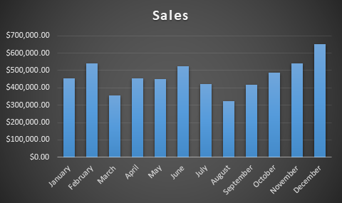
In this lesson you will learn how to find the style number of an Excel chart using VBA. Let’s consider this sample Excel sheet. This Excel sheet lists the number of sales for a few different items. Then an Excel chart has been used to visualize the sales of each item.

Now let’s see how we can find the style number of this Excel chart using VBA. I will show you how to find the style number of an active chart and of a chart by its name. In the first example you will be able to find the style number of a selected chart.

Find style number of an active chart using VBA

In this example we are going to find the style number of an active chart. To find the style number from this method, first click on the chart you want to find the style number of.

Then run this simple subroutine.

Sub FindChartStyleNo_Method1()

     MsgBox ActiveChart.ChartStyle

End Sub

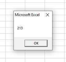
This is the result obtained from the subroutine.

Find the style number of a chart by its name using VBA

From the previous subroutine we were able to get the style number of an active chart. You may know that each chart of a worksheet has a name. So in this next VBA macro we are going to find the style number of an Excel chart by its name. Remember that these names are not unique. Because users can create multiple charts with the same name.

Don’t know how to find the name of a chart? Check this post.
Find the name of a chart in Excel

Now let’s look at how to find the style number of a chart by its name. Assume that the name of our chart is “Chart 1”. Then we can find the style number of the chart using the following simple VBA macro.

Sub FindChartStyleNo_ByName()

     Dim MyChart As Chart

     Set MyChart = ActiveSheet.Shapes("Chart 1").Chart

     Debug.Print MyChart.ChartStyle

End Sub

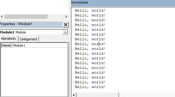
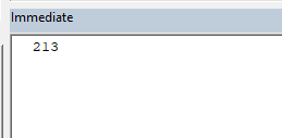
If we run the above macro the style number of the Excel chart will be printed in the immediate window like this.

In this next example you will learn how to go through all the charts in the worksheet and print their names and style numbers. Here is the example sheet I’m going to use.

Let’s name this subroutine as FindChartStyleNo_AllCharts

Sub FindChartStyleNo_AllCharts()

End Sub

We need two variables for this subroutine.

Dim WS As Worksheet
Dim Sh As Shape

Next we can assign the worksheet to the WS variable as follows.

Set WS = Worksheets("Sales data")

Now we need to iterate through all the shapes of the worksheet. We can use For Each statement to do that.

For Each Sh In WS.Shapes

Next

Inside the For Each loop we need to separate only the charts. Because lots of other objects also belong to this shapes collection. So here we are going to use an If statement and the “Shape.Name” property to distinguish charts from other objects. Once charts are extracted then we can print the name and the style number in the immediate window.

If InStr(1, Sh.Name, "Chart", vbTextCompare) > 0 Then
     Debug.Print "Chart name - "; Sh.Name & " Style Number - " & Sh.Chart.ChartStyle
End If

So here is the full code of this subroutine.

Sub FindChartStyleNo_AllCharts()

     Dim WS As Worksheet
     Dim Sh As Shape

     Set WS = Worksheets("Sales data")

     For Each Sh In WS.Shapes
          If InStr(1, Sh.Name, "Chart", vbTextCompare) > 0 Then
               Debug.Print "Chart name - "; Sh.Name & " Style Number - " & Sh.Chart.ChartStyle
          End If
     Next

End Sub

This is the result of the above subroutine

But this method will only work when the user hasn't changed the chart name manually. If it is possible for the user to change the chart names then you can use the “Shapes.Type” property instead of the “Shapes.Name”. This is how you can modify the If statement section to use “Shapes.Type” property.

If Sh.Type = 3 Then
     Debug.Print "Chart type - "; Sh.Type & " Style Number - " & Sh.Chart.ChartStyle
End If

3 is the MsoShapeType value that represents the charts. Check below article from Microsoft documentation to see the values for different types of shapes.

MsoShapeType enumeration (Office)